Delay estimation by FFT

Code snippet

This article relates to the Matlab / Octave code snippet: Delay estimation with subsample resolution
It explains the algorithm and the design decisions behind it.

Introduction

There are many DSP-related problems, where an unknown timing between two signals needs to be determined and corrected, for example, radar, sonar, time-domain reflectometry, angle-of-arrival estimation, to name a few. It is not difficult to find solutions in the literature - a good starting point is for example the list of references in [1] - but for some reason things are never as easy in the lab as they look on paper.
This article describes an algorithm that has served me well in the past. It can cope with relatively long signals (millions of samples), works regardless of the absolute delay, positive or negative and is relatively robust, accurate and fast.
For example, it can be used to line up baseband signals that represent input and output of a power amplifier, to extract distortion characteristics by coherent processing.

Use cases, advantages and disadvantages

• Use as general-purpose tool for simulations and measurements to align input and output samples
• For example: It has been used extensively for wide-band radio frequency measurements, which require very accurate input-/output alignment.
• Notuseful for real-time applications. The whole signal needs to be known in advance.
• Notrecommended for hardware or embedded implementation. Use a specialized method and optimize for the signal in question.
• Meant as a robust lab tool that (usually) does what it's supposed to do without need for any further supervision.
• Properly used, the accuracy can be orders of magnitude higher than typical "ad-hoc" solutions. It sure beats lining up signals with an oscilloscope.
• Suitable for band pass (high pass) test signals, gaps in the power spectrum and narrow-band interference
• May fail as result of excessive group delay variations (see Figure 6 why).
  If so, my code snippet [5] may be a more reliable but slower and less accurate alternative.
• I wouldn't recommend it for timing-recovery 'homework' problems where the estimation is the main objective (if so: For some down-to-earth introduction, see [4] ).
  That said, it will happily give arrival time, magnitude and carrier phase from a known preamble / pilot signal, for example to calibrate the delay in a link-level simulator.

Accuracy

In theory, any delay estimator is limited by the Cramér-Rao bound [2], which depends largely on the shape of the power spectrum and the signal-to-noise ratio. In the absence of noise and distortion - easily simulated in Matlab - numerical accuracy remains the main limiting factor, and for example nano-sample accuracy can be achieved.
No formal proof has been carried out. If needed, it is straightforward to set up an artificial example with known delay, or to compare real-world results with a "true" maximum-likelyhood estimator such as [3] (that may however be less suited for everyday use).

Background: Cyclic signals

It is assumed that input- and output signals are cyclic. In other words, the observed signal period is one cycle of a repetitive test signal where the system is in steady state, with all transients settled. If needed, this can be approximated by zero-padding the signals in the time domain to arbitrary length.
The assumption of cyclic signals is quite important, as it allows to convert freely between time- and frequency domain, and to evaluate the underlying continuous-time waveform anywhere between samples without loss of information besides arithmetic errors..
Note that the result can become heavily biased if either signal has been truncated, relative to the other one. This lies in the nature of the problem and is not related to this specific algorithm: The optimum delay is "pulled" towards the direction that maximizes the general overlap between waveforms.

Background: Delaying bandlimited signals

Delaying a signal by a fraction of a sample reveals additional points on the continuous-time equivalent waveform in the same way as an ideal reconstruction filter, as found in the definition of the Nyquist limit. Now if the signal is zero at some sampling instants, this does not automatically mean it would be also zero between samples.
All too often, delaying an abrupt step will show a lot of "ringing" - the ringing has been there all the time, but remained invisible, as long as the signal was observed only on the original sampling grid.
The first Nyquist criterion guarantees that there will be no interaction from one sample to another - but it says nothing about the times in-between.

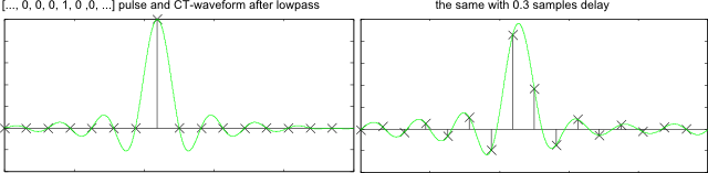
Figure 1: A pulse, its continuous-time equivalent (green) and the result of time-delaying

Algorithm

Figure 2 shows the algorithm in a nutshell:

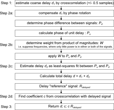
Figure 2: Overview of the algorithm

Step 1: Coarse timing estimation by crosscorrelation

A well-known solution to estimate delay is to calculate the cross-correlation between the two signals. An efficient implementation calculates |ifft(fft(a) .* fft(b)|, using FFT for cyclic convolution.
A peak in the result indicates the integer-sample delay with best alignment.
Crosscorrelation provides the coarse estimate (integerDelay) in the code snippet. Figure 3 shows an example:

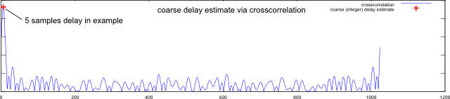
Figure 3: Coarse estimate by crosscorrelation

The coarse estimate for the delay is found by peak search. Unfortunately, most real-life delays don't fall onto an integer sampling grid.
If so, the error can be made arbitrarily small by oversampling, in other words by zero-padding fft(a) and fft(b) at the center.
There are two drawbacks:

• Timing resolution and FFT size scale proportionally, making high accuracy computationally expensive
• The correlation peak is relatively shallow, and numerical accuracy becomes a bottleneck when searching for the maximum.

Step 2: Fine estimation via slope of relative phase

Instead, delay estimation is done in the frequency domain, where a time delay results in a linearly increasing phase shift and its slope indicates the delay. The slope will be extracted by linear regression.

Phase ambiguity

A delay of one sample causes a phase shift of pi at the highest frequency: For delays greater than one sample, the phase wraps around, as only a principal value of the angle of a complex number is known. This ambiguity needs to be resolved:

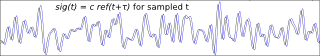
Fig. 4 illustrates the relative phase between both signals over frequency, assuming a delay of several samples.
The phase wraps around, which prevents finding its slope via linear regression.

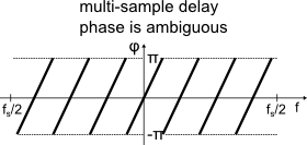
Figure 4: Relative phase between signals for multi-sample delay

Step 2a: Coarse correction

Now the coarse delay estimate (Figure 3) is removed from the signal by phase-shifting.
As long as the remaining unknown delay is less than +/- 0.5 samples, the relative phase is now confined in a +/- pi window, and no phase wrapping will occur:

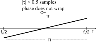
Figure 5: Relative phase between signals after coarse correction. Remaining delay is fractional-sample.

This approach will fail, if frequency-dependent group delay variations cause the phase to wrap at some frequency.
This may happen for example when dealing with a multipath radio channel: "Determining the delay" is not a well-defined problem, once the group delay varies with frequency.
In this case, phase unwrapping may be able to correct the problem, as long as it does not introduce any unwrapping errors. If necessary, set enableUnwrap = true (by default disabled).

Figure 6: Failure by wrap-around from group delay variations

When dealing with transmitters, receivers, test equipment and the like, the signal chain is usually designed with a constant group delay in mind, and the method is quite reliable. With channel models or signals on the band edge of a filter, your mileage may vary.

After coarse correction, the phase should not wrap around anymore, and linear regression will correctly determine its slope.

Step 2b: Weighted phase

At any frequency, the relative importance of the phase depends on the power of either signal: For example, the phase is meaningless both if no power is received and also if no power was transmitted (as the received signal is obviously useless in this case).
Therefore, the phase is scaled with the product of signal power at each bin.

Step 2c: Linear regression

A least-squares solution is found by projecting the phase on a basis formed by a constant term and a linear-phase term, the latter corresponding to a unit delay. As the phase has been weighted, the same weights are applied to the basis.
The resulting coefficient of the linear-phase term is the remaining delay in samples, which is summed with the coarse delay to give the final delay estimate.

Step 2d: Scaling factor

Finally, one signal is delayed by the delay estimate, and projected onto the other signal. A scaling factor c results.

Step 3: Return values

The function returns the delay estimate, the scaling factor c and a replica of the second signal that has been shifted and scaled to match the first signal.

Advanced use

Some comments on using the function in real-world applications:

Error vector

The shifted / scaled replica of the second signal can be subtracted from the first signal. The residual can be considered "vector error", or signal energy in an output signal that cannot be "'explained" by the input signal. It may reveal unwanted artifacts even though they are buried below a strong wanted signal, for example extract the noise floor from a modulated signal.

Error vector spectrum

Especially the spectrum of the error vector can lead to interesting insights. My spectrum analyzer code snippet can be a useful tool to investigate:
Figure 7 shows an example of actual measurement data on a radio frequency amplifier:

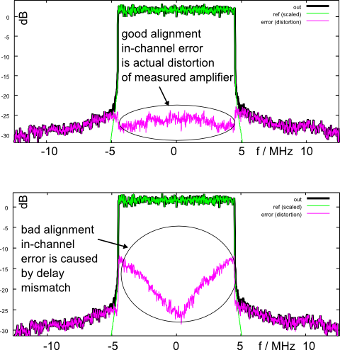
Figure 7: Example vector error spectrum

In short, the green trace shows the input signal to a power amplifier, and the black trace the output signal. Subtracting the time-aligned and scaled input from the output reveals distortion products both within and outside the wanted channel bandwidth of +/- 5 MHz. The in-channel distortion becomes visible only after removing the wanted signal itself.
In the lower picture, an artificial delay of 7 ns was introduced before subtracting the signals. The delay mismatch causes an error that obscures the distortion products, particularly at higher frequencies. This example illustrates the need for accurate delay compensation in wideband measurements.
If the error vector spectrum increases with frequency in a V-shape, it is a sign for delay misalignment or frequency mismatch of radio frequency carriers. A typical cause is that a measurement instrument returns n+1 samples for a time period that should result only in n samples. The same will happen if radio frequency generator and analyzer don't use a common reference clock.

Phase unwrapping?

Finally, some words on phase unwrapping, which is a commonly used solution in frequency domain delay estimation:
Detect, where the relative phase between neighboring samples changes by more than pi, and correct with a multiple of 2 pi:

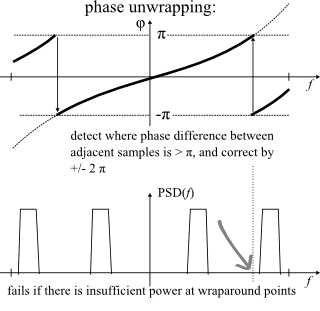
Figure 8: Phase unwrapping

If the signal-to-noise ratio over the unwrapping range is consistently high, all is well.
Unfortunately, only one noisy frequency sample within the signal bandwidth may cause an unwrapping error, leading to catastrophic failure.
Typical causes are:

• AC coupling or DC offset compensation, i.e. removal of carrier leakage around 0 Hz in a radio receiver
• Multi-channel signals with guard bands between channels
• Signals with narrow-band test tones (sine waves)
• narrow-band interference inside a wideband signal

Phase unwrapping is implemented in the code snippet, but disabled by default. Set enableUnwrap = true to turn it on, and set enableCoarseCorr = false to disable the coarse correction and rely solely on phase unwrapping.

References

[1] Y. Zhang; W. H. Abdulla: A Comparative Study of Time-Delay Estimation Techniques Using Microphone Arrays

[2] Wikipedia: Cramér-Rao Bound

[3] Moddemeijer, R., An information theoretical delay estimator

[4] Signal Processing in Telecommunications 2: Course notes

[5] Code snippet: Delay estimation revisited

Would you like to be notified by email when Markus Nentwig publishes a new blog?