Spline interpolation

• Matlab
• FPGA
• Verilog

A cookbook recipe for segmented y=f(x) 3^rd-order polynomial interpolation based on arbitrary input data.
Includes Octave/Matlab design script and Verilog implementation example.

Keywords: Spline, interpolation, function modeling, fixed point approximation, data fitting, Matlab, RTL, Verilog

Introduction

Splines describe a smooth function with a small number of parameters.
They are well-known for example from vector drawing programs, or to define a "natural" movement path through given points in computer animation.
They are an engineer's tool, apparently originating from the shipbuilding industry, with widespread use documented from world war II to make "backup copies" of aircraft design templates that did not fit into a bomb shelter.

Splines are convenient to model arbitrary continuous functions, as fixed-point implementation is efficient and straightforward. In DSP applications, a spline's continuous first derivative helps to confine interpolation error close to frequencies of the signal, which is often desirable (i.e. to limit audio aliasing to higher frequencies where the ear is more sensitive). For example, Catmull-Rom splines are commonly used for low-cost audio resampling.

This article provides a recipe to construct spline coefficients from arbitrary scattered points via a least-squares solver.
For practical design problems this allows a fluid "cooking-style" design process, where the result is shaped by adding (or removing) input data to control the approximation error.

Figure 1: Spline approximation of a function, possibly from noisy data

The splines discussed in this article consist of multiple 3^rd-order polynomial sections.
Transitions between segments are continuous both in value and in the first derivative, resulting in a function that is for most practical purposes fairly "smooth".

Examples

The example in figure 2 is a logarithmic volume control curve from a DIY FPGA project. Using four segments, the spline approximation is virtually indistinguishable from the original exponential function. The approximation error is well below 1 percent (-40 dB).

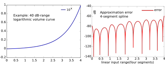
Figure 2: A four-segment spline modeling a 40 dB-range volume curve

A second example (figure 3) shows a spline fit to noisy and non-gridded data.
It originates from the same project, where the target waveform represents three cycles of a Hammond organ drawbar signal, with noise added both to sampled values (y axis) and sampling time instants (x axis).
As can be seen, the design process is robust towards irregularities in the data.

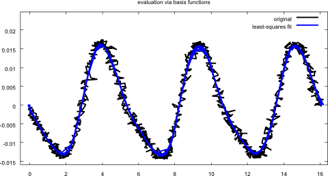
Figure 3: 16-segment spline through a very noisy Hammond organd drawbar sample

The math

For segmentation, the input variable is split into an integer part and a fractional part (figure 4).

Figure 2: A four-segment spline modeling a 40 dB-range volume curve

For a number of segments that is a power of two, the separation is done by taking the higher- and lower bits.
The Verilog implementation below shows the details for signed numbers.
Each of the segments is described by a polynomial y(x) = a₀+a₁x+a₂x²+a₃x³ with x in a domain interval -1..1 covering the segment (see "polynomial variable" in figure 4).

Within a segment, four basis functions p₁.. p₄ are defined that have zero value and zero slope at x = +/-1, with the exception of

• p₁ has value 1 at x = -1
• p₂ has value 1 at x = 1
• p₃ has slope 1 at x = -1
• p₄ has slope 1 at x = -1

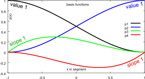
Figure 5: Basis functions

For each support point, a first scaling factor is assigned to a pair of basis functions p₁, p₂ on the left and right side of the support point, respectively: The scaling factor controls the value of the spline at the support point, but does not affect the slope (because the slope of both p₁, p₂ is zero at the support point). This is shown in the upper half of Figure 6.
In a similar manner, a second scaling factor is assigned to p₃, p₄ to set the slope, without affecting the value at the support point (lower half of Figure 6).

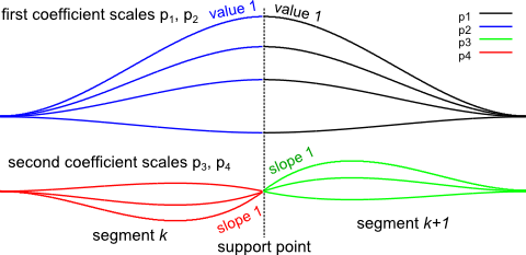
Figure 6: Scaled basis functions enforcing continuity through a support point

The scaling factors are then found by minimizing the difference between input data and approximation in a least-squares problem.
Finally, the polynomial coefficients for each spline segment are determined by summing up all four scaled basis function polynomials.
The derivation for the basis functions in Maxima CAS can be found here.

Number of support points

To span n segments, n+1 support points are needed.
Relevant for all practical purposes is the number of segments, not support points, as each segment defines one set of polynomial coefficients.
For example, a fixed-point implementation may use four MSBs to select one of 16 segments. The equation system in the design process will use 17 support points.
In the provided Matlab program, the outermost support points do not need any special consideration with regard to continuity: In an interval without input data, any basis function becomes invisible to the least-squares cost function.

Octave (Matlab) script

All the little details are taken care of in the Octave / Matlab program, which can be downloaded here.
Several examples to generate data are included. A spline is generated, evaluated and plotted.
Finally, fixed-point coefficients are written to a file that is imported by the Verilog RTL implementation.

RTL implementation

This Verilog implementation demonstrates the evaluation of the spline in RTL. It was written with the 18-bit multipliers on Spartan-6 FPGAs in mind.

Input variable

The signed input is first converted to offset binary by inverting the sign bit.
The four MSBs become the index into the coefficient table. The LSBs are then converted back in the same manner from offset binary to two's complement signed.

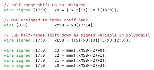
Figure 7: Fixed-point handling of input variable

Multiply-accumulate

With four MSBs stripped off, the LSB part of the input variable contains 13 fractional bits. After multiplication with the LSB part, arithmetic right shift by 13 bits restores the decimal point. Prior to that, 0.5 LSB is added for correct midpoint rounding.

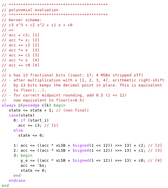
Figure 8: Horner scheme evaluation

In the Verilog code, the four operations of the Horner scheme evaluation are written out explicitly for clarity.
Alternatively, a MAC could be used, with the feedback path opened during the first cycle to load c₃ (i.e. "CLR" input).

Simulation result

The simulation snapshot in figure 9 covers the whole 18-bit input range of input values.
The segment structure is clearly visible in MSB, LSB and the selected coefficients (see figure 7), and the output signal looks as expected.

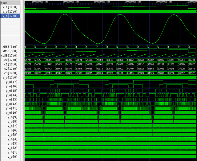
Figure 9: Simulation result for "Hammond drawbar" spline

Pipelined RTL implementation

A second RTL version ( download) is a pipelined implementation of the four-segment volume curve example from Figure 2. The evaluation of four independent input variable values is interleaved.
The pipelining generally allows higher clock frequencies by introducing additional delay.

Numerical accuracy

The implementations are not bit-exact because of intermediate rounding after every multiplication. A typical error is one LSB in the output.

Conclusion

This article presents a design method to construct an interpolation function in fixed-point RTL from arbitrary data.
A spline is derived via a least-squares fit. The spline is then evaluated using the Horner scheme.
This work was originally done for an open-source FPGA synth project. If it gets reused (amplifier model, anybody?), I'd be happy to hear about it.

Download

The whole project archive, including the links from the text, can be downloaded here.

Sign in