Complex Down-Conversion Amplitude Loss

This blog illustrates the signal amplitude loss inherent in a traditional complex down-conversion system. (In the literature of signal processing, complex down-conversion is also called "quadrature demodulation.")

The general idea behind complex down-conversion is shown in Figure 1(a). And the traditional hardware block diagram of a complex down-converter is shown in Figure 1(b).

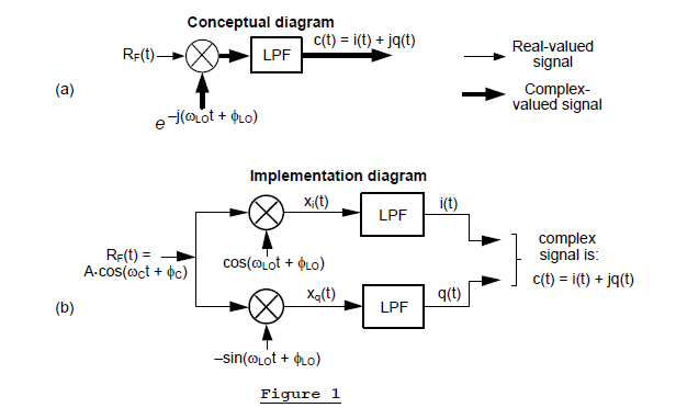
Let's assume the input to our down-conversion system is an analog radio frequency (RF) signal, \(R_F(t)\), defined as:

$$ R_F(t) = A \cdot cos(\omega_ct + \phi_c)\tag{1} $$

where \(A\) is the cosine wave's peak amplitude, \(\omega_c = 2\pi f_c\) is the carrier frequency in radians/sec., \(\phi_c\) is the cosine wave's initial phase angle measured in radians, and \(t\) is our time variable measured in seconds.

In Figure 1(b) the subscript LO means 'local oscillator' where \(\omega_{LO} = 2\pi f_{LO}\) is the local oscillator's frequency in radians/sec. and \(\phi_{LO}\) is the oscillator's initial phase angle measured in radians.

Algebraic Form of Output c(t)

To begin determining the amplitude loss of the output \(c(t)\) relative to the \(R_F(t)\) input, we analyze Figure 1(b) as follows:

$$ x_i(t) = R_F(t) \cdot cos(\omega_{LO}t + \phi_{LO})\\\ = A \cdot cos(\omega_ct + \phi_c) \cdot cos(\omega_{LO}t + \phi_{LO}).\tag{2} $$

Using the \(cos(a)cos(\beta)\) trigonometric product identity, we can write Eq. (2) as:

$$ x_i(t) = A \cdot [cos(\omega_ct + \phi_c -\omega_{LO}t -\phi_{LO}) \\ + cos(\omega_ct + \phi_c + \omega_{LO}t + \phi_{LO})]/2 \\ = A \cdot [cos((\omega_c -\omega_{LO})t + \phi_c -\phi_{LO}) \\ + cos((\omega_c + \omega_{LO})t + \phi_c + \phi_{LO})]/2. \tag{3} $$

Notice that \(x_i(t)\) comprises a low-frequency sinusoid and a high-frequency sinusoid. And both sinusoids have peak amplitudes that are one half the peak amplitude of \(R_F(t)\) in Eq. (1).

In a similar way, we can represent Figure 1(b)'s \(x_q(t)\) as:

$$ x_q(t) = R_F(t) \cdot [-sin(\omega_{LO}t + \phi_{LO})] \\ = A \cdot cos(\omega_ct + \phi_c) \cdot [-sin(\omega_{LO}t + \phi_{LO})]. \tag{4} $$

Using the \(cos(\alpha)sin(\beta)\) trigonometric product identity, and keeping Eq. (4)'s minus sign in mind, we can write Eq. (4) as:

$$  x_q(t) = A \cdot [-sin(\omega_ct + \phi_c + \omega_{LO}t + \phi_{LO}) \\ + sin(\omega_ct + \phi_c -\omega_{LO}t -\phi_{LO})]/2 \\= A \cdot [-sin ((\omega_c + \omega_{LO})t + \phi_c + \phi_{LO}) \\ + sin((\omega_c -\omega_{LO})t + \phi_c -\phi_{LO})]/2. \tag{5} $$

Like \(x_i(t)\), \(x_q(t)\) comprises a low-frequency sinusoid and a high-frequency sinusoid where both sinusoids have peak amplitudes equal to one half the \(A\) peak amplitude of \(R_F(t)\) in Eq. (1).

Assuming the lowpass filters in Figure 1(b) have passband gains of one (unity), and they completely eliminate the high-frequency sinusoids in \(x_i(t)\) and \(x_q(t)\), we can describe the filters' outputs as:

$$ i(t) = A \cdot cos((\omega_c -\omega_{LO})t + \phi_c -\phi_{LO})/2 \tag{6} $$ and $$ q(t) = A \cdot sin((\omega_c -\omega_{LO})t + \phi_c -\phi_{LO})/2. \tag{7} $$

Both \(i(t)\) and \(q(t)\) are real-valued signals. Again, the above derivation is based on the assumption that the lowpass filters in Figure 1(b) have infinite attenuation in their stopbands!

Complex Down-Conversion Output Notations

In rectangular notation, our down-converter's \(c(t)\) output is represented by:

$$ c(t) = i(t) + jq(t) \\ = (A/2)[cos((\omega_c -\omega_{LO})t + \phi_c -\phi_{LO}) \\ + jsin((\omega_c -\omega_{LO})t + \phi_c -\phi_{LO})]. \tag{8} $$

In polar notation, our down-converter's \(c(t)\) output is represented by:

$$ c(t) = {A\over 2} e^{j[\omega_c-\omega_{LO})t + \phi_c - \phi_{LO}]} \tag{9} $$

So our final output is a complex exponential whose magnitude is always \(A/2\), its frequency is \(\omega_c-\omega_{LO}\) radians/sec., and it's phase angle (at t = 0) is \(\phi_c-\phi_{LO}\) radians.

• Scenario #1: When \(\omega_{LO} = \omega_c \) and \(\phi_{LO} = \phi_c\), the \(c(t)\) output is a real-valued constant equal to A/2. (\(i(t) = A/2\) and \(q(t) = 0\).)

• Scenario #2: When \(\omega_{LO} = \omega_c\) and \(\phi_{LO} ≠ \phi_c\), the \(c(t)\) output is a complex-valued constant whose magnitude is equal to A/2, and whose phase angle is a constant \(\phi_c‑\phi_{LO}\) radians.

• Scenario #3: When \(\omega_{LO} < \omega_c\) the \(c(t)\) output is a complex exponential, whose magnitude is equal to A/2 rotating counterclockwise on the complex plane at a rate of \(\omega_c‑\omega_{LO}\) radians/second. (Output signals \(i(t)\) and \(q(t)\) are quadrature-related real-valued sinusoids, having peak amplitudes of A/2, whose frequencies are both \(\omega_c‑\omega_{LO}\) radians/second.)

Don't Be Fooled When Estimating Signal Amplitude Loss

It's common, the first time we use software to model our down-conversion process, to plot and examine the amplitudes of discrete versions of the \(R_F(t)\), \(i(t)\), and \(q(t)\) signals. When \(\omega_{LO} < \omega_c\) our time-domain plots will show that both \(i(t)\) and \(q(t)\) have peak amplitudes that are half the peak amplitude of \(R_F(t)\). Seeing that, it's easy to fall into the trap of thinking, "Ah ha. Output amplitude losses by a factor of two. The down-converter's output amplitude loss measured in decibels (dB) must be -6 dB."

That approach is incorrect. The following shows the correct way to determine the dB loss of our down-converter.

Complex Down-Conversion Signal Loss

The dB loss of output \(c(t)\) relative to the input \(R_F(t)\) in our Figure 1(b) down-conversion process is:

dB loss of \(c(t) = \) 

$$ 10 log_{10}{\left({Power \, of \, c(t)}\over {Power \, of \, R_F(t)}\right)}\tag{10} $$

From Eq. (9)

$$ Power \, of \, c(t) = c(t) \cdot c^*(t) \\ = {A \over 2}e^{j[(\omega_c-\omega_{LO})t + \phi_c - \phi_{LO}]} \cdot  {A \over 2}e^{-j[(\omega_c-\omega_{LO})t + \phi_c - \phi_{LO}]} \\ = (A/2)^2 \cdot e^{j0} = (A/2)^2 = A^2/4 $$

where '*' means conjugate. And we know that the power of the \(R_F(t)\) input cosine wave is:

Power of \(R_F(t) = A^2/2\).

Then from Eq.(10), our complex down-converter's true signal loss is:

$$ dB \, loss \, of \, c(t) = 10 log_{10} \left({A^2/4}\over {A^2/2} \right) = 10 log_{10} \left(1\over 2 \right) = -3 \, dB. \tag{11} $$

To depict the average signal powers, P, within our down-converter, I present Figure 2. (A dash-line ellipse indicates a dual-path complex signal.) There we see that the average power of the \(c(t)\) output is one half the average power of the \(R_F(t)\) input.

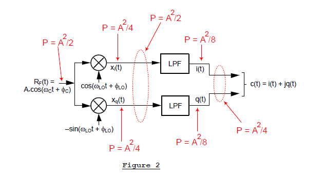
Figure 2 tells us that the complex down-converter's signal power loss of 3 dB is caused by the lowpass filtering and not by the complex frequency translation.

Software Modeling a Down-Conversion System

If you decide to model the Figure 2 down-conversion process in software, know that your \(c(t)\) output magnitude results will not correspond exactly with the above equations. That's due to the difficulty in implementing ideal lowpass filters having infinite attenuation in their stopbands. In addition, real-world filters suffer from "start up transient" behavior until their output sequences reach a steady state time-domain response.

When you model a down-conversion system using software it's common to plot the discrete Fourier transform (DFT) spectra of various signals within the system's signal paths. You do that to ensure that your frequency-translated, or filtered, signals have the expected spectral content.

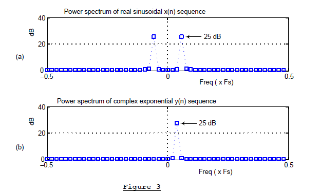
But comparing the average power of various signals is a bit tricky using spectral data. For example, Figure 3(a) shows the spectral power, measured in dB, of an arbitrary real-valued sinusoidal \(x(n)\) time sequence. (Ten times the log ₁₀ of squared spectral magnitudes.) Figure 3(b) shows the spectral power of an arbitrary \(y(n)\) complex exponential time sequence. Because the spectral peaks are all the same in that figure you might naively assume that the average powers of \(x(n)\) and \(y(n)\) are equal to each other. They are not! (The average power of \(y(n)\) is one half the average power of \(x(n)\).)

Rather than trying to compare signal average powers based on spectral dB data, I suggest you plot your various down-converters' signals in the time-domain. And then examine, and compare, their instantaneous amplitudes or magnitudes.

Of course, the most reliable way to compare the average power of two time signals is to compute each signal's average signal power, over N time samples, using:

$$ Average \, power \, of \, x(n) = {1 \over N} \sum_{n=0}^{N-1}\lvert x(n)\rvert^2 \tag{12} $$

where time index n is: n = 0,1,2,...N-1. Equation (12) is valid for both real-valued or complex-valued \(x(n)\) signal sequences. Once you have the average power values of two signals you can determine their power ratio, measured in dB, using Eq. (10).

Lyons Ranting and Raving

There's one last point I want to make here. More than once I've seen documents graphically depicting complex down-conversion as shown in Figure 4.

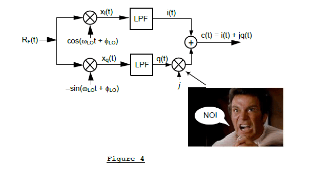
It's simply incorrect to show the implementation of the 'j' operator as a hardware multiplication. In addition, it makes no sense to show a hardware adder summing a purely real-valued signal with what appears to be a purely imaginary-valued signal to produce a complex-valued signal.

So, ...if you ever write a document presenting a traditional complex down-conversion hardware block diagram I strongly suggest you use the dual-output Figure 2 rather than Figure 4.

Sign in