Understanding and Implementing the Sliding DFT

• Tips and Tricks
• DFT_FFT

Introduction

In many applications the detection or processing of signals in the frequency domain offers an advantage over performing the same task in the time-domain.   Sometimes the advantage is just a simpler or more conceptually straightforward algorithm, and often the largest barrier to working in the frequency domain is the complexity or latency involved in the Fast Fourier Transform computation.   If the frequency-domain data must be updated frequently in a real-time application, the complexity and latency of the FFT can become a significant impediment to achieving system goals and keeping cost and power consumption low.  Many modern applications, like medical imaging, radar, touch-screen sensing, and communication systems, use frequency-domain algorithms for detecting and processing signals.  In many implementations complexity or power consumption must be kept low while minimizing latency.  The Sliding DFT algorithm provides frequency domain updates on a per-sample basis with significantly fewer computations than the FFT for each update.

First, The Math

The derivation of the Sliding DFT is reasonably straightforward and shows exact equivalence to the DFT, i.e., there is no loss of information or distortion tradeoff with the Sliding DFT algorithm compared to a traditional DFT or FFT.  The derivation is shown here for completeness, but disinterested readers can skip this section and not lose too much sleep.

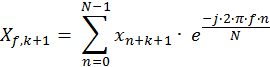
The basic assumption for using a Sliding DFT is that a long time-domain stream exists over which a shorter transform window will be slid.    This is essentially what happens with a spectrogram, where a length-N transform is taken at regular intervals in a long or continuous stream of time-domain samples.  For the derivation of the Sliding DFT we assume that a transform is taken with every new time-domain sample, so that the length-N transform window moves along the time domain stream a sample at a time.  The input stream with samples x_k, where k runs over an index with a range larger than N, can then yield a length-N transform at every k^th sample.   Using the traditional definition of the DFT we can write this k^th transform as follows, where f is the frequency index and n the time index within the length-N transform window:

Eq. 1

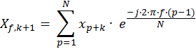
The next transform in the sliding sequence will be the (k+1)th and can be rewritten as:

Eq. 2

A simple trick can now be done which allows a rearrangement of the terms.   We can substitute p = n+1 into Eq. 2, with the range of p therefore 1 to N, instead of 0 to N-1 for n.   The computations are the same as before, just with a different index definition.

Eq. 3

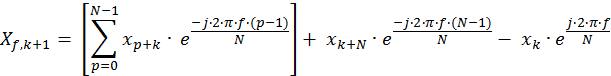
The Nth term can be taken out of the summation and added separately.  At the same time we can introduce a zeroth term in the summation, as long as we subtract it again outside of the summation.   The resulting equation is inelegant, but useful:

Eq. 4

The common term can be factored out as follows:

Eq. 5

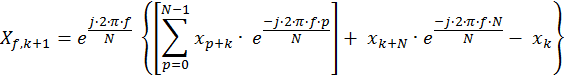
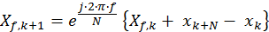
In Eq. 5 the exponential with the x_k+N term can never have a value other than 1+j0 since f always has integer values, and so can be eliminated.  The summation, in the square brackets, is the DFT of the k^th vector with p as an index instead of n.  Equation 5 can therefore be rewritten as:

Eq. 6

The Algorithm

Equation 6 shows the derived expression for the Sliding DFT.  The frequency bins of the (k+1)^th transform, X_f,k+1, are computed recursively from the bins of the k^th transform X_f,k.   For each desired frequency bin with index f, the difference of the newest time-domain input sample, x_k+N, and the oldest sample in the DFT window, x_k, is added to the bin.   The result is then multiplied by the bin-frequency-dependent exponential term, e^-j2pf/N, to produce the updated output for that bin.

The advantages compared to using an FFT are readily apparent.   For each transform the update requires  one complex addition, x_k+N - x_k, that is common to all bins,  and one complex multiplication and addition for each output bin.   If the input stream, x, is real-valued, then only the initial addition is real-valued.  Only the desired output bins need to be computed since there is no interdependence between bins, and the transform window can be any length N rather than only powers of two.   Compare this to log₂(N) stages of N/2 butterfly operations for an FFT, where essentially all of the N outputs must be computed regardless of how many are actually needed.    Figure 1 shows a signal flow diagram of an implementation of Equation 6.  The initial delay and addition is common to all bins, and the recursive complex multiply and accumulation stage is repeated for each frequency bin to be computed.

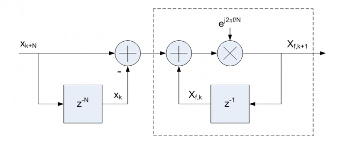
Figure 1.   Signal flow diagram of the Sliding DFT as expressed in Equation 6.  The boxed portion is repeated for each unique value of f.

The computational advantage of the Sliding DFT may diminish if a new transform is not needed with every input sample, e.g., if a transform is only needed every M input samples, and all output bins are computed, the computation order would be O(N×M) rather than O(N×log₂(N)) for the FFT.   The Sliding DFT will still provide an advantage in latency in all cases, however, since after the Mth input each output bin can be computed with only two complex-valued operations once x_k+N - x_k is computed. 

Initialization

The recursive nature of the Sliding DFT algorithm means that some initialization method is required.  The output X_f,k+1 is only valid if X_f,k was valid, and each output relies on inputs from N previous samples.  There are two common methods for initializing the algorithm:

1. Cycle zeroes in to flush the delay lines before cycling in data.   Similarly, if the buffer registers are resettable, resetting the signal path memory to zero before cycling data in accomplishes the same thing.  After N data samples have been cycled in the output will be valid. 

2. The N cycle initialization delay in the first method can be avoided by initializing all X_f,k with an FFT of the previous N input samples.  In some systems, especially off-line applications, this may provide an advantage.

Numeric Stability

In applications where the computations are performed with integer or fixed-point arithmetic, truncation or rounding of the e^-j2pf/N coefficients can result in a complex coefficient magnitude greater than unity.  In these cases the corresponding X_f,k output may become unstable and experience growth from self-excitation.  Usually a simple fix for this condition is to subtract an LSB from the largest component, either I or Q, of the offending coefficient which should bring the coefficient magnitude back to less than or equal to unity.

Conclusion

Under certain common circumstances the Sliding DFT provides computational and latency advantages over the FFT with no loss of information or added distortion.  The computational advantage can be significant, providing a reduction in complexity and/or power consumption when compared to the use of an FFT.  Similarly, in real-time applications the reduction in latency can be critical to system performance.  

References

[1] T. Springer. "Sliding FFT computes frequency spectra in real time", EDN Magazine, Sept. 29, 1988, pp. 161-170.

[2] E. Jacobsen and R. Lyons. "The Sliding DFT", IEEE Signal Processing Magazine, Mar. 2003, pp. 74-80.

[3] E. Jacobsen and R. Lyons. "An update to the Sliding DFT", IEEE Signal Processing Magazine, Jan. 2004, pp. 110-111.

[4] E. Jacobsen and R. Lyons, "Sliding Spectrum Analysis," Ch. 14 in Streamlining Digital Signal Processing: A Tricks of the Trade Guidebook (Paperback), Richard G. Lyons (Editor), Wiley-IEEE Press, 2007, pp. 145-157

[5] Richard S. Lyons, Understanding Digital Signal Processing, Prentice-Hall, 3rd Ed., 2010

Sign in