Approximating the area of a chirp by fitting a polynomial

• Basics
• Python
• Tutorials

Once in a while we need to estimate the area of a dataset in which we are interested. This area could give us, for example, force (mass vs acceleration) or electric power (electric current vs charge).

One way to do that is fitting a curve on our data, and let's face it: this is not that easy. In this post we will work on this issue using Python and its packages. If you do not have Python installed on your system, check here how to proceed.

Specifically, we will need:

• Numpy: the numerical basis for Python scientific software.
• Scipy: tons of scientific functions for different applications.
• Matplotlib: a nice plot platform.

We can import these packages on Python using the code below.

import numpy as np
import scipy as sp
import matplotlib.pyplot as plt

We used the form import package as nickname to avoid typing the entire package name. Note that we got only pyplot from matplotlib, which provides a MATLAB-like plotting framework. Then, we use np, sp and plt instead of numpy, scipy and matplotlib.pyplot respectively.

On our example, let's calculate the area of a chirp. Scipy's function signal.chirp is an easy function to generate a chirp varying in time. This is its general form:

sp.signal.chirp(t, f0, t1, f1, method='linear', phi=0, vertex_zero=True)

Where:

• t is an array containing the time points of interest.
• f0 is the frequency at time equals to zero.
• t1 is the time at which f1 is specified.
• f1 is the frequency of the waveform at t1.
• method is the kind of frequency sweep. We can use 'linear', 'quadratic', 'logarithmic', and 'hyperbolic'. When we do not provide a value, the default value is 'linear'.
• phi is the phase offset in degrees. The default value is zero.
• vertex_zero is used only when method='quadratic', and determines whether the vertex of the generated parabola is at t=0 or t=t1.

Check more information about signal.chirp on the scipy online documentation. You can also type sp.signal.chirp? on your preferred Python prompt.

Let's generate a chirp. First, we generate a time interval using the numpy's function linspace. Its general form follows:

np.linspace(start, stop, num=50, endpoint=True, retstep=False, dtype=None)

Where:

• start is the starting value of the sequence.
• stop depends on endpoint. It is the end value of the sequence.
• num is an natural number, meaning the number of samples to generate. The default number is 50.
• endpoint decides if stop is within the sequence (endpoint=True) or not. The default value is True.
• retstep, when true, returns the number of samples and the space between them. The default value is False.
• dtype specifies the data type of the output array. If it is not given, linspace will infer the data type from the other input arguments.

More information about linspace is given at the scipy online documentation. You can also type np.linspace? on your Python prompt.

On our example, the time interval begins on 0 and ends on 10. It has 100 samples. The following code generates this interval and stores it on the time_interval variable.

time_interval = np.linspace(0, 10, num=100)

Now, using time_interval, let's generate our chirp. Its values of f0, t1 and f1 are 0, 1 and 1, respectively. We will generate a quadratic chirp, using method='quadratic'. This code generates this chirp and stores its points on example_chirp.

example_chirp = sp.signal.chirp(time_interval, 0, 1, 1, method='quadratic')

Let's visualize this chirp. In order to do that we use matplotlib.pyplot's stem function, which plots a discrete sequence of data using vertical lines and symbols. Its general form follows:

plt.stem(y, linefmt='b-', markerfmt='bo', basefmt='r-')<span></span>

Where:

• y are the data points.
• linefmt modifies the color and appearance of the vertical lines. The default value is 'b-', which plots lines blue-colored ('b') and continuous ('-').
• markerfmt modifies the marker positioned at the value (x, y). The default value is 'bo', which plots blue ('b') circles ('o').
• basefmt modifies the horizontal line plotted at 0. The default value is 'r-', which plots a line red ('r') and continuous ('-').

Check also for stem at the matplotlib documentation, or type plt.stem? on your Python prompt.

Let's use plot the chirp using stem's default values. We use the following code:

plt.stem(time_interval, example_chirp)

The figure representing our discrete chirp is given on Figure 1.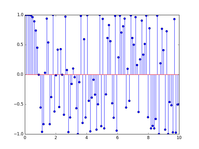 Figure 1. Our example chirp, generated from sp.signal.chirp and plotted using plt.stem.

Now we will fit a curve on this chirp. On this example we use Chebyshev's polynomials, that can be fitted on a dataset using numpy's polyomial.Chebyshev.fit function. There are many alternatives, such as Legendre, Laguerre and Hermite. Check these possibilities at the scipy online documentation.

The simplest form of polynomial.Chebyshev.fit follows:

np.polynomial.Chebyshev.fit(x, y, deg)

Where:

• x are the x-coordinates of the sample points.
• y are the y-coordinates of the sample points.
• deg is the degree of the polynomial to be fitted.

For more information and arguments to this function, please check the scipy documentation. As an alternative, type np.polynomial.Chebyshev.fit? on your Python prompt.

To show the behavior of this function, we will use three different arguments for deg: 20, 45 and 115. The following code will generate these different polynomials based on our data and store them on the variables cheby_chirp20, cheby_chirp45 and cheby_chirp115.

cheby_chirp20 = np.polynomial.Chebyshev.fit(time_interval, example_chirp, deg=20)
cheby_chirp45 = np.polynomial.Chebyshev.fit(time_interval, example_chirp, deg=45)
cheby_chirp115 = np.polynomial.Chebyshev.fit(time_interval, example_chirp, deg=115)

Let's plot these results. Note that the results of polynomial.Chebyshev.fit are functions, not points; we need to provide the plot interval as an argument. We plot these three polynomials against the original data as subplots. They will be represented as green lines ('g') with width equals to 2 (lw=2). We also add a label to each of them, which will appear on the legend of each plot. Check the matplotlib examples for more ideas on subplots.

f, ax_array = plt.subplots(3, sharex=True)
ax_array[0].stem(time_interval, example_chirp)
ax_array[0].plot(time_interval, cheby_chirp20(time_interval), 'g', lw=2, label='cheby deg 20')
ax_array[0].legend()
ax_array[1].stem(time_interval, example_chirp)
ax_array[1].plot(time_interval, cheby_chirp45(time_interval), 'g', lw=2, label='cheby deg 45')
ax_array[1].legend()
ax_array[2].stem(time_interval, example_chirp)
ax_array[2].plot(time_interval, cheby_chirp115(time_interval), 'g', lw=2, label='cheby deg 115')
ax_array[2].legend()

The three generated polynomials can be seen on Figure 2.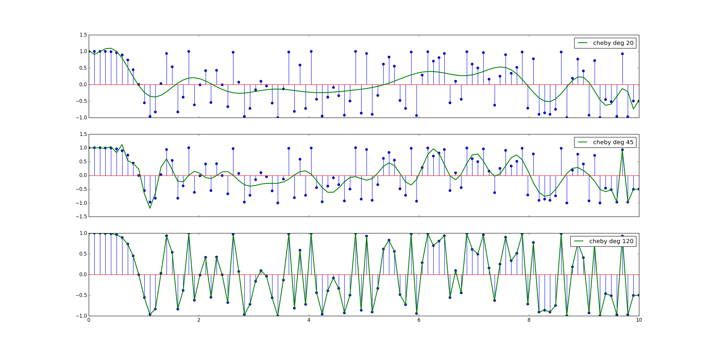

Figure 2.: Three polynomials representing our data, obtained using np.polynomial.Chebyshev.fit.

Now, let's use scipy's integrate.quad function to calculate the area of these polynomials. This function uses a technique from QUADPACK, a Fortran library. The simplest form of integrate.quad is given below:

scipy.integrate.quad(func, a, b)

Where:

• func is the function to be integrated.
• a is the lower limit of integration.
• b is the upper limit of integration.

This function returns the integral value and the absolute error in the result. For more information on integrate.quad, its arguments and usage examples, check the scipy documentation. You can also type sp.integrate.quad? on your Python prompt.

Let's define the integration interval between zero and pi. Then, we integrate the three polynomials. Check the code below:

integ_int = [0, np.pi]
cheby20_area, cheby20_err = sp.integrate.quad(cheby_chirp20, *integ_int)
cheby45_area, cheby45_err = sp.integrate.quad(cheby_chirp45, *integ_int)
cheby115_area, cheby115_err = sp.integrate.quad(cheby_chirp115, *integ_int)

We define integ_int and pass it to integrate.quad using the star (*), which provides the arguments all at once to the function. For example, on the cheby_chirp20 case, this is an alternative to:

cheby20_area, cheby25_err = sp.integrate.quad(cheby_chirp20, 0, np.pi)

We need to present area and error now. This can be done using print, which provides a nice output:

print('The area of cheby20 in this interval is {0}. The absolute error is {1}'.format(cheby20_area, cheby20_err))
print('The area of cheby45 in this interval is {0}. The absolute error is {1}'.format(cheby45_area, cheby45_err))
print('The area of cheby115 in this interval is {0}. The absolute error is {1}'.format(cheby115_area, cheby115_err))

The function print presents a message. Using format we can also present the variable values on {0}, {1}, {2}, and so on. More on the print function can be seen on the Python documentation. As always, you can type print? on your Python prompt.

Let's check the results:

The area of cheby20 in this interval is 0.4637693754972824. The absolute error is 1.5334233932461724e-13
The area of cheby45 in this interval is -8.792912670367262. The absolute error is 2.9585315540800773e-12
The area of cheby115 in this interval is 151230239254.8722. The absolute error is 50.06303513050079

The two first polynomials wielded acceptable results, but there is something wrong about cheby_chirp115. We can confirm that checking its absolute error (around 50). Let's see what is going on, plotting the integration areas of these polynomials.

We define the integration interval with 50 points using linspace to plot the results. This interval will be attributed to integ_full. Again, we will use plt.subplots:

integ_full = np.linspace(*integ_int)
f, ax_array = plt.subplots(3, sharex=True)
ax_array[0].stem(time_interval, example_chirp)
ax_array[0].plot(time_interval, cheby_chirp20(time_interval), 'g', lw=2, label='cheby deg 20')
ax_array[0].fill_between(integ_full, cheby_chirp20(integ_full), color='orchid', label=r'$\int_{0}^{\pi}\,$cheby_chirp20(x)')
ax_array[0].legend()
ax_array[1].stem(time_interval, example_chirp)
ax_array[1].plot(time_interval, cheby_chirp45(time_interval), 'g', lw=2, label='cheby deg 45')
ax_array[1].fill_between(integ_full, cheby_chirp45(integ_full), color='orchid', label=r'$\int_{0}^{\pi}\,$cheby_chirp45(x)')
ax_array[1].legend()
ax_array[2].stem(time_interval, example_chirp)
ax_array[2].plot(time_interval, cheby_chirp115(time_interval), 'g', lw=2, label='cheby deg 115')
ax_array[2].fill_between(integ_full, cheby_chirp115(integ_full), color='orchid', label=r'$\int_{0}^{\pi}\,$cheby_chirp115(x)')
ax_array[2].legend()

We employed plt.fill_between to plot the integration areas. For comparison, we plotted also the original points and the polynomials. Note that we added LaTeX code to the label; it is necessary to add an r before the string. The areas of integration are shown on Figure 3.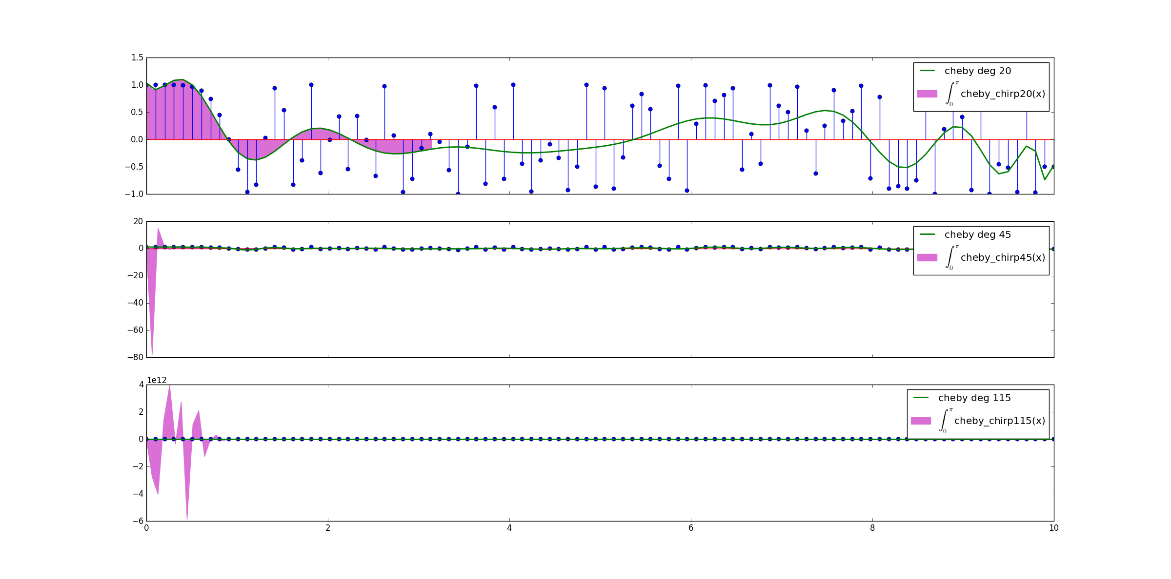

Figure 3. The integration areas highlighted on the fitted polynomials.

Check how the integration interval of cheby_chirp115 is messy! cheby_chirp45 is not good too. cheby_chirp20 is satisfactory from 0 to 1 approximately, but we need more than that on the rest of our data.

Lesson learned: be careful choosing the degree of the fitted polynomial! Lower degrees may not represent your data nicely; however, higher degrees may lead to a poor conditioned fit. The solution could be to search for a good balance.

All right, this is it! Hope you enjoyed this post. Are there anything wrong? Do you have any ideas to improve it? Please share them with us! Also, you can download the codes on GitHub.

Thank you for joining us! See you next time!

Additional notes:

• jms_nh proposed another tools for fitting the chirp: "The waveforms you've shown really aren't very polynomial-like and would be better handled by curve-fitting using cubic splines or Savitsky-Golay filtering". He has a point: according to the SciPy documentation, "Fits using Chebyshev series are usually better conditioned than fits using power series, but much can depend on the distribution of the sample points and the smoothness of the data. If the quality of the fit is inadequate splines may be a good alternative".

Sign in