Compressive Sensing - Recovery of Sparse Signals (Part 1)

• Basics
• Academia / Research

The amount of data that is generated has been increasing at a substantial rate since the beginning of the digital revolution. The constraints on the sampling and reconstruction of digital signals are derived from the well-known Nyquist-Shannon sampling theorem. To review, the theorem states that a band-limited signal, with the highest frequency of $f_{max}$, can be completely reconstructed from its samples if the sampling rate, $f_{s}$, is at least twice the signal bandwidth. If the Nyquist-Shannon criteria is not satisfied then any frequency component greater than $f_{s}/2$ will become indistinguishable from a lower frequency component (i.e. aliasing).

Although the Nyquist-Shannon criteria gives a concrete formula for recovery of bandlimited signals, it is becoming increasingly impractical to implement due to ever-increasing size of data being generated. For example, high-resolution images taken from modern image sensors cause a lot of burden on communication channels, or in some cases, the communications channels are inadequate for efficient data transfer [1]. Due to increasing impracticality, a lot of research in the past decade has been focused on the recovery of signals from far fewer samples than required by the Nyquist-Shannon sampling criteria.

Before going any further, it is important to formulate a mathematical definition of signal acquisition and recovery process. Signal acquisition can be stated as a classical linear algebra problem

$$y = Ax$$

where $y \in \mathbb{R}^{m}$ or $y \in \mathbb{C}^{m}$ is the measured signal vector, $x \in \mathbb{R}^{m}$ or $x \in \mathbb{C}^{m}$ is the unknown signal vector, and $A \in \mathbb{R}^{m \times n}$ or $A \in \mathbb{C}^{m \times n}$ is measurement or "sensing'' matrix. For example, $y$ could be a vector obtained through spectral (fourier) measurement of audio signal, in which case the vector would consist of fourier coefficents of the signal $x$, and $A$ would be a fourier transformation matrix. In the signal recovery process, the objective is to find to unknown signal vector $x$ given $y$ and $A$. So the signal recovery requires solving the inverse problem

$$x = A^{-1}y$$

In traditional signal processing, $A$ is a full rank matrix, and $m$ is typically much larger than $n$ so that $x$ can be recovered with high fidelity (i.e. over-determined system). However, the problem of interest is to recover $x$ from far fewer samples than required by the Nyquist-Shannon criteria, or when $m << n$ (i.e. under-determined system). It turns out that if signals are structured in a certain way, then it is possible, at least in theory, to recover signals from fewer samples than suggested by the Nyquist-Shannon theorem. One set of signals that can theoretically be recovered from far fewer samples are signals that are sparse. Mathematically, a signal is said to be $k$-sparse when it has at most $k$ non-zeros

$$\Sigma_{k} = {x: |supp(x)| \leq k}$$  

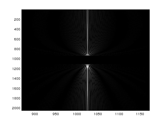
where $supp(x)$ is the support of vector $x$ and $|supp(x)|$ denotes the cardinality of the set of points where x is non-zero. An example of $k$-sparse signal is the fourier transform of the Shepp-Logan phantom image, which is a standard test image in medical signal processing. The fourier transform of the test image is given below.

Figure 1: Shepp-Logan test image.

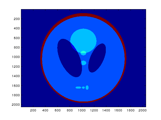
Figure 2: FFT of the Shepp-Logan test image. Due to the sparse nature of the fourier transform, the fourier coefficients are non-zero over a very small area.

If the signal $x$ is k-sparse then it only has $k$ degrees of freedom and it could, in principle, be uniquely determined from $m << n$ measurements if certain requirements are met. The complete mathematical form of these requirements can be found in [4]. For brevity, I will just paraphrase the requirements as follows

1. $x$ can be uniquely reconstructed from $y$ if the $m \times n$ matrix $A$ is such that every set of $2k$ columns of $A$ are linearly independent.
2. The lower bound on dimensionality of $y$ is $m \geq Ck\log(\frac{n}{k})$, where constant $C \approx 0.28$.

$x$ can be uniquely reconstructed by solving the following well-known convex optimisation problem

$$minimise \; |x|_{1}\\subject \;to \;Ax=y $$

where $|x|_{1}$ is l-1 norm. The problem is also known as basis pursuit. 

This is a very brief theoretical background of sparse signal recovery, which is also known as "compressed" or "compressive" sensing (CS). In my next blog post, I will demonstrate sparse recovery by providing a simulation. [Hopefully, that would be more interesting.]

[Side-note: I realise that it's not easy to wrap one's head around the formulation of signal acquisition and recovery as a classical linear algebra problem ($y=Ax$), since $x$ is typically an analog signal and I am representing it using a discrete vector. I will clarify this in a future post, but for now, the reader can get some background information from lectures on compressive sensing available at [2,3].]

[1] DARPA ARGUS super high-resolution camera (https://en.wikipedia.org/wiki/ARGUS-IS)

[2] Yonina Elder's lecture on CS ()

[3] Richard Burbank's lecture CS (http://youtube.com/watch?v=RvMgVv-xZhQ)

[4] Eldar, Yonina C., and Gitta Kutyniok, eds. Compressed sensing: theory and applications. Cambridge University Press, 2012.

Sign in