Differentiating and integrating discrete signals

• Free ebooks
• Python
• DFT_FFT

I am back at work on Think DSP, adding a new chapter on differentiation and integration.  In the previous chapter (which you can read here) I present Gaussian smoothing, show how smoothing in the time domain corresponds to a low-pass filter in the frequency domain, and present the Convolution Theorem.

In the current chapter, I start with the first difference operation (diff in Numpy) and show that it corresponds to a high-pass filter in the frequency domain.  I use historical stock prices as an example, where we can think of the closing price each day as a signal, and the daily changes as the first difference of the sample.

I compute the first difference using convolution in the time domain and multiplication in the frequency domain, and confirm that the result is the same (within floating point error).  All the details are in this IPython notebook.

Integration and cumulative sum

In the next step, I show that the first difference operation approximates the first derivative, and compute the filter for the derivative.

Up to this point, all of the examples behave as expected.  But when I get to integration, I find some things I don’t understand -- I hope some readers will be able to help me out.

First I compute the integration filter and confirm that it is the inverse of the differentiation filter.  So far, so good.

Then I show that the cumulative sum (cumsum in Numpy) is the inverse of diff.  To find the filter that corresponds to cumsum, I find the filter that corresponds to diff and invert it.  To check the result, I take a signal and its cumulative sum, take the FFT of both, and compute the ratios of corresponding amplitudes.  These ratios (shown in gray) should at least approximate the inverse diff filter (dark blue):

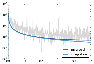
In fact they have the same general shape, but the ratios are noisy and look like they are offset by a constant factor (a shift on a log scale).  So that’s PUZZLE #1: what’s going on there?

An actual periodic signal

I suspect that part of the problem is that the signal I’m using is not really periodic.  To test that theory, I tried the whole thing again with a sawtooth.

Again, I compute the FFT of both the signal and its cumulative sum, then compute the ratios of the amplitudes.  This time the ratios (in red) correspond exactly to the inverse diff filter (in gray), as expected.

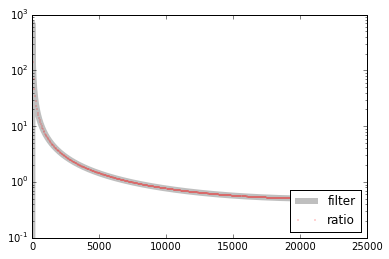
So that’s better.

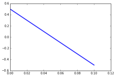
My next step is to find the window that corresponds to this filter.  The result is a straight line (so that happens to be a sawtooth signal):

In theory, convolving with this window in the time domain should correspond to applying the inverse diff filter in the frequency domain, which should correspond to applying the cumsum operation in the time domain.  But here’s what I get:

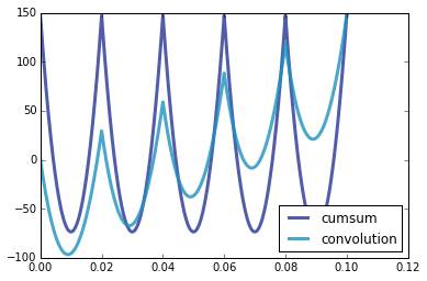
The light dark blue line is the cumulative sum of the original sawtooth signal.  The light blue line is the convolution of the sawtooth with the window in the previous figure.  They are not the same, so that’s PUZZLE #2: why not?

One issue is that the version computed with cumsum starts at 150 and the convolution starts at 0.  But that’s not really a problem: it’s just because I unbiased the cumulative sum; if I don’t do that, they both start at 0.

The other issue is that the convolution has a trend that shouldn't be there, and a smaller peak-to-peak amplitude. In terms of frequencies, it looks like there's a lot of energy at a very low frequency, and energy has been leaked from the higher frequencies.

I have a tentative theory that the problem is related to the behavior of 1/f near zero.  In this range, the discrete approximation is pretty terrible, which might account for strange behavior at very low frequencies.  But that’s as far as I got. If anyone has hints about what’s going on, I am all ears.

Again, all the details are in this IPython notebook.

If both puzzles get solved, I will explain the solutions in my next post (and probably in the book, too).  Thanks for reading!

Sign in