Exponential Smoothing with a Wrinkle

• Basics
• DFT_FFT
• Tutorials

Introduction

This is an article to hopefully give a better understanding to the Discrete Fourier Transform (DFT) by providing a set of preprocessing filters to improve the resolution of the DFT. Because of the exponential nature of sinusoidal functions, they have special mathematical properties when exponential smoothing is applied to them. These properties are derived and explained in this blog article.

Basic Exponential Smoothing

Exponential smoothing is also known as exponential averaging. The definition is straight forward. Suppose you have a sequence of values denoted as $ S_n $, then exponential smoothing produces another sequence using the simple formula:

$$ F_0 = S_0 \tag 1 $$

$$ F_n = b S_n + a F_{n-1} \tag 2 $$

Where $ a $ and $ b $ are scalar parameters having values between 0 and 1, and $ a + b = 1 $.

This definition is true for all values of $ n $, so $ n-1 $, $ n-2 $, etc., can be substituted in for n.

$$ F_{n-1} = b S_{n-1} + a F_{n-2} \tag 3 $$

Plugging (3) into (2) gives an expanded version of the definition.

$$ F_n = b S_n + a \left( b S_{n-1} + a F_{n-2} \right) \tag 4 $$

Using the definiton for $ n- 2 $, the expanded version can be expanded further.

$$ F_n = b S_n + a \left( b S_{n-1} + a \left( b S_{n-2} + a F_{n-3} \right) \right) \tag 5 $$

Now a pattern starts to emerge. All the summation terms except the last one have a factor of $ b $, which can be factored out.

$$ F_n = b \left( S_n + a S_{n-1} + a^2 S_{n-2} \right) + a^3 F_{n-3} \tag 6 $$

The series formed by the pattern can be put in summation form.

$$ F_n = b \sum_{k=0}^{2} { a^k S_{n-k} } + a^3 F_{n-3} \tag 7 $$

Repeating the pattern, assuming that $ |a| < 1 $ and all the $ S_n $ values are bounded, the series will converge when it is extended to infinity.

$$ F_n = b \sum_{k=0}^{\infty} { a^k S_{n-k} } \tag 8 $$

The exponential value of $ a^k $ is what gives the average its name.

Backward Exponential Smoothing

If the sequence represents time series values, then ascending subscript values represent moving forward in time. If the data has already been collected, as in a audio signal buffer, or any other after the fact collection, then the basic definition can be reversed.

$$ B_{N-1} = S_{N-1} \tag 9 $$

$$ B_n = b S_n + a F_{n+1} \tag {10} $$

The backward definition can be expanded in a manner similar to the forward case with the only difference being the sign of the iteration variable $(k)$ in the subscript of the sequence value.

$$ B_n = b \sum_{k=0}^{\infty} { a^k S_{n+k} } \tag {11} $$

Cancelling the Lags

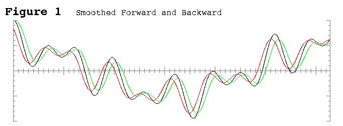
One of the properties of exponential averages is that the average value represents the values in the near past. Thus, the average looks like it lags the signal. By symmetry, in the backward case, the lag is reversed and actually leads the signal when viewed in an ascending subscript manner. These effects can be seen in Figure 1. The black line is a sample signal, the green line is the forward exponential average, and the red line is the backward exponential average.

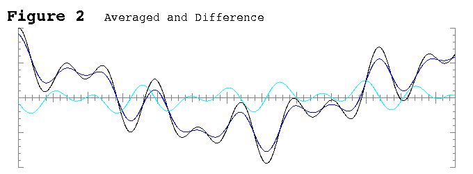
When the leading and trailing exponential averages are combined with an arithmetic average, the lags cancel themselves out on symmetric features of the signal. This can be seen in the blue line in Figure 2.

$$ A_n = ( B_n + F_n ) / 2 \tag {12} $$

First Derivative Like Behavior

Here is the wrinkle. When the difference is taken, instead of the sum, in the combination, the result acts a lot like a first derivative of the averaged values. This can be understood conceptually be realizing that the leading lag represents the expected value of the signal from the near future and the trailing lag represents the expected value of the signal from the near past. If the future value is higher than the past value, the signal is on an upward trend. If the future value is lower than the past value, the signal is on a downward trend. Just like with a derivative, if the future value is the same as the past value, the signal is horizontal. In a varying signal, this means either at a peak, a trough, or a horizontal inflection point. This can be seen in the cyan line in Figure 2.

$$ D_n = ( B_n - F_n ) / 2 \tag {13} $$

Sinusoidal Signal

A sinusoidal signal is a very special case of a time varying signal. Because it represents a pure tone when the signal is an audio signal, the sinusoidal case is very important in Digital Signal Processing (DSP). A pure tone signal can be modelled mathematically as:

$$ S_n = M cos ( f \cdot { 2\pi \over N } n + \phi ) \tag {14} $$

Where $ N $ is the number of points in a sample frame, $ f $ is the frequency in cycles per frame, $ M $ is the amplitude, and $ \phi $ is the phase shift.

For convenience, a variable ($\alpha$) can be defined to simplify the definition.

$$ \alpha = f \cdot { 2\pi \over N } \tag {15} $$

$$ S_n = M cos ( \alpha n + \phi ) \tag {16} $$

In practical applications, $ \alpha $ can be assumed to range from 0 to $ \pi $. A value of zero is the so called DC (direct current) case where the value of the signal remains constant. A value of $ \pi $ occurs at the Nyquist frequency, which is the limit of resolution for a DFT.

Exponential Smoothing of a Sinusoidal Signal

The definition of the signal (16) can be plugged into the forward exponential average series (8).

$$ F_n = b \sum_{k=0}^{\infty} { a^k M cos \left( \alpha ( n - k ) + \phi \right) } \tag {17} $$

With a little algebra, the argument of the cosine function can be rearranged to separate the $ n $ and the $ k $ values.

$$ F_n = M \cdot b \sum_{k=0}^{\infty} { a^k cos ( \alpha n + \phi - \alpha k ) } \tag {18} $$

The cosine expression can then be expanded by using the cosine angle addition formula.

$$ F_n = \\ M \cdot b \sum_{k=0}^{\infty} { a^k \left[ cos( \alpha n + \phi )cos( \alpha k )  + sin( \alpha n + \phi )sin( \alpha k ) \right] } \tag {19} $$

A similar treatment can be applied in the backward case.

$$ B_n = \\ M \cdot b \sum_{k=0}^{\infty} { a^k \left[ cos( \alpha n + \phi )cos( \alpha k )  - sin( \alpha n + \phi )sin( \alpha k ) \right] } \tag {20} $$

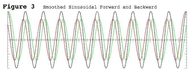
The forward and backward exponential averages of a sinusoidal signal are shown in Figure 3.

When the averaged sequence is calculated, the sine terms cancel each other out.

$$ A_n = M \cdot b \sum_{k=0}^{\infty} { a^k \left[ cos( \alpha n + \phi )cos( \alpha k ) \right] } \tag {21} $$

Since the $ n $ based cosine expression is independent of the summation iterator, it can be factored out of the summation.

$$ A_n = M cos( \alpha n + \phi ) \cdot b \sum_{k=0}^{\infty} { a^k cos( \alpha k ) } \tag {22} $$

The expression on the left of the dot is the definition of the original signal. The expression on the right of the dot is only dependent on the smoothing factor and the frequency. Notably, it is independent of the amplitude or phase of the signal, and it is independent of the sequence subscript. For a given frequency, the expression on the right will be the same for all subscript values. This means it is a multiplier of the signal. Since exponential averaging smooths down bumps, the multiplier is positive and has a value less than one. Therefore it can be called a dampening factor.

This proves that for a sinusoidal signal, the forward and backward lags do indeed cancel each other out exactly.

The same treatment can be applied to the difference case, the distinction being the cosine terms get cancelled and the sine terms remain.

$$ D_n = -M \cdot b \sum_{k=0}^{\infty} { a^k \left[ sin( \alpha n + \phi )sin( \alpha k ) \right] } \tag {23} $$

$$ D_n = -M sin( \alpha n + \phi ) \cdot b \sum_{k=0}^{\infty} { a^k sin( \alpha k ) } \tag {24} $$

Just like the averaged case, the expression on the left of the dot is a sinusoidal, and the expression on the right is a dampening factor.

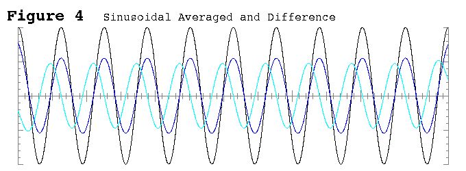
The averaged and difference cases are shown in Figure 4.

Closed Form Equation for the Averaged Case

The summation in the dampening factors are a bit unwieldy. With a little bit of work the summation can be eliminated and replaced with a closed form expression.

Here is where the exponential nature of the sinusoidal functions comes into play.

$$ cos( \theta ) = { e^{ i \theta } + e^{ -i \theta } \over 2 } \tag {25} $$

The definition in (25) can be plugged into the summation expression of (22).

$$ \sum_{k=0}^{\infty} { a^k cos( \alpha k ) } = { 1 \over 2 } \sum_{k=0}^{\infty} { a^k ( e^{ i \alpha k } + e^{ -i \alpha k } ) } \tag {26} $$

The sum inside the summation allows the summation to be broken out as two geometric series summations.

$$ \sum_{k=0}^{\infty} { a^k cos( \alpha k ) } = { 1 \over 2 } \left[ \sum_{k=0}^{\infty} { ( a e^{ i \alpha } )^k } + \sum_{k=0}^{\infty} { ( a e^{ -i \alpha } )^k } \right]\tag {27} $$

The summation formula for an infinite geometric series can now be applied.

$$ \sum_{k=0}^{\infty} {x^k} = { 1 \over { 1 - x } } \tag {28} $$

$$ \sum_{k=0}^{\infty} { a^k cos( \alpha k ) } = { 1 \over 2 } \left[ { 1 \over { 1 - a e^{ i \alpha } } } + { 1 \over { 1 - a e^{ -i \alpha } } } \right] \tag {29} $$

The summations have now been eliminated. The fractions inside the brackets can be added to make a single fraction.

$$ \sum_{k=0}^{\infty} { a^k cos( \alpha k ) } = { 1 \over 2 } \left[ { 2 - a e^{ i \alpha } - a e^{ -i \alpha } } \over { 1 - a e^{ i \alpha } - a e^{ -i \alpha } + a^2 } \right] \tag {30} $$

The exponential definition of a cosine (25) can now be used in reverse, twice. The result is a simplified summation expression.

$$ \sum_{k=0}^{\infty} { a^k cos( \alpha k ) } = { { 1 - a cos \alpha } \over { 1 - 2 a cos \alpha + a^2 } } \tag {31} $$

Plugging the summation expression back into (22) and replacing $ b $ with $ ( 1 - a ) $ gives a final closed form expression for the averaged smoothing of a sinusoidal signal.

$$ A_n = M cos( \alpha n + \phi ) \cdot { { ( 1 - a ) ( 1 - a cos \alpha ) } \over { 1 - 2 a cos \alpha + a^2 } } \tag {32} $$

Interestingly, the denominator in the dampening expression is in the form of the Law of Cosines.

Closed Form Equation for the Difference Case

A closed form expression for the difference case can be derived in a similar manner to the average case. Since it is sine based, the exponential definition of the sine function is needed.

$$ sin( \theta ) = { e^{ i \theta } - e^{ -i \theta } \over 2 i } \tag {33} $$

The sine definition can then be substituted into the summation expression.

$$ \sum_{k=0}^{\infty} { a^k sin( \alpha k ) } = { 1 \over {2i} } \sum_{k=0}^{\infty} { a^k ( e^{ i \alpha k } - e^{ -i \alpha k } ) } \tag {34} $$

The summation can be split into two geometric series summations.

$$ \sum_{k=0}^{\infty} { a^k sin( \alpha k ) } = { 1 \over {2i} } \left[ \sum_{k=0}^{\infty} { ( a e^{ i \alpha } )^k } - \sum_{k=0}^{\infty} { ( a e^{ -i \alpha } )^k } \right]\tag {35} $$

The infinite geometric series summation formula can be applied to each summation.

$$ \sum_{k=0}^{\infty} { a^k sin( \alpha k ) } = { 1 \over {2i} } \left[ { 1 \over { 1 - a e^{ i \alpha } } } - { 1 \over { 1 - a e^{ -i \alpha } } } \right] \tag {36} $$

The difference of the two fractions in the brackets can be calculated.

$$ \sum_{k=0}^{\infty} { a^k sin( \alpha k ) } = { 1 \over {2i} } \left[ { a e^{ i \alpha } - a e^{ -i \alpha } } \over { 1 - a e^{ i \alpha } - a e^{ -i \alpha } + a^2 } \right] \tag {37} $$

The sine and cosine exponential definitions can be used to simplify the fraction.

$$ \sum_{k=0}^{\infty} { a^k sin( \alpha k ) } = { { a sin \alpha } \over { 1 - 2 a cos \alpha + a^2 } } \tag {38} $$

Finally, the summation expression can be replaced in the difference case (24).

$$ D_n = -M sin( \alpha n + \phi ) \cdot { { ( 1 - a ) a sin \alpha } \over { 1 - 2 a cos \alpha + a^2 } } \tag {39} $$

Comparison with the Derivative

If the signal (16) was defined as a function instead of a sequence, then the derivative could be taken.

$$ { dS \over dn } = -M sin( \alpha n + \phi ) \cdot \alpha \tag {40} $$

The similarity to (39) is apparent. When $ \alpha $ is small, which corresponds to many samples per cycle, the similarity is almost a proportional equivalence. When $ \alpha $ is small, $ sin( \alpha ) $ is roughly equal to $ \alpha $, and $ cos( \alpha ) $ is roughly equal to one.

$$ { { ( 1 - a ) a sin \alpha } \over { 1 - 2 a cos \alpha + a^2 } } \approx { { ( 1 - a ) a } \over { 1 - 2 a + a^2 } } \alpha = { { a } \over { 1 - a } } \alpha \tag {41} $$

When $ a $ has a value of 1/2, and $ \alpha $ is small, the difference case (39) becomes nearly equivalent to the derivative (40).

Amplitude Dampening of Smoothed Sinusoidal Signals

How much dampening occurs is a function of the smoothing parameter $ a $ and the frequency of the sinusoidal, represented by $ \alpha $. Figure 5 shows the dampening effect as a function of $ \alpha $ for five sample values of $ a $. The values are .1, .3, .5, .7, and .9. The higher the $ a $ value, the more dampening there is and the lower the curve on the graph. No matter what the smoothing parameter is, DC values (the far left axis) remain unscathed. As expected, higher frequency values are more impacted by smoothing than lower ones at any level of smoothing.

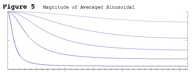
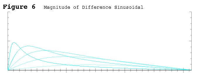
Figure 6 shows the dampening effect in the difference case. DC values are completely obliterated. The proportionality to $ \alpha $ when $ \alpha $ is small can be clearly seen in the graph. The steeper the line the higher the smoothing parameter. Note that the proportionality extends much further along the $ \alpha $ axis for the lower values of $ a $. Unlike the average case, high frequencies near the Nyquist limit (the far right axis) are also zeroed out.

In either case, the smoothing effect is local in the time domain, so noise gets dampened similarly to high frequency components.

Conclusion

The combination of exponential smoothing and the exponential nature of sinusoidal functions allows improved performance of the DFT by reducing the effects of noise and allowing the selection of frequency ranges to be emphasized. The frequency is preserved in both the averaged and difference cases. The phase is preserved in the average case and shifted by a quarter cycle ( $ \pi / 2 $ ) in the difference case. The original magnitude can be found by dividing the recovered magnitude by the dampening factor for the known frequency and smoothing factor. This allows the DFT to be used in a much more targeted, noise resistant way.

Appendix. Sample Python Implementation

import numpy as np

#========================================================================
def main():

#---- Set parameters

        N = 50
        
        M     = 5.678
        alpha = 1.234
        phi   = 2.345
        
        a = 0.50

#---- Allocate the Arrays

        S = np.zeros( N )   # Signal
        F = np.zeros( N )   # Forward
        B = np.zeros( N )   # Backward
        A = np.zeros( N )   # Average
        D = np.zeros( N )   # Difference

#---- Fake a Signal

        for n in range( N ):
          S[n] = M * np.cos( alpha * n + phi )

#---- Forward Pass

        b = 1.0 - a
        
        F[0] = S[0]
        
        for n in range( 1, N ):
          F[n] = b * S[n] + a * F[n-1]
          
#---- Backward Pass

        B[N-1] = S[N-1]
        
        for n in range( N-2, -1, -1 ):
          B[n] = b * S[n] + a * B[n+1]
        
#---- Results Pass

        for n in range( 1, N ):
          A[n] = ( B[n] + F[n] ) * 0.5
          D[n] = ( B[n] - F[n] ) * 0.5
          
#---- Print Results

        for n in range( N ):
          TheDerivative = - alpha * M * np.sin( alpha * n + phi )
          
          print "%2d %10.4f %10.4f  %10.7f %10.7f" % \
          ( n, S[n], TheDerivative, A[n] / S[n], D[n] / TheDerivative )

#========================================================================
main()

Sign in