Amplitude modulation and the sampling theorem

• Audio DSP
• Basics
• Communication

I am working on the 11th and probably final chapter of Think DSP, which follows material my colleague Siddhartan Govindasamy developed for a class at Olin College.  He introduces amplitude modulation as a clever way to sneak up on the Nyquist–Shannon sampling theorem.

Most of the code for the chapter is done: you can check it out in this IPython notebook.  I haven't written the text yet, but I'll outline it here, and paste in the key figures.

Convolution with impulses

I start with an example that demonstrates convolution with a series of impulses: it adds up shifted, scaled copies of the original wave, as shown here:

You can hear what it sounds like in the IPython notebook.

Amplitude modulation

Then I show an example of amplitude modulation in four steps (from top to bottom):

1) The spectrum of the original wave.

2) After multiplying by a cosine carrier wave at 10 kHz, the spectrum is shifted by plus and minus 10 kHz.

3) After demodulating by multiplying by the same carrier wave, each of the copies splits and shifts again, adding up in the middle.

4) By filtering out the high-frequency peaks at plus and minus 20 kHz, we can recover the original signal.

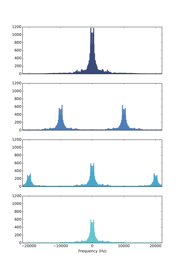
To understand how that works, we can look at the spectrum of the carrier wave: it has impulses at plus and minus 10 kHz.  When we multiply in the time domain, we are convolving in the frequency domain.  And as we saw in the first example, convolving with impulses makes shifted, scaled copies.  In the first example it makes copies of the wave; in this example it makes copies of the spectrum.

Sampling

Next we see what happens when we sample a signal.  I start with a recording sampled at 44.1 kHz, keep every 4th sample, and set the other samples to 0.  This simulates the effect of sampling the original signal at about 11 kHz.

Here's what happens in the frequency domain: the top spectrum is the 44 kHz wave; the bottom spectrum is the 11 kHz wave after downsampling:

1) The top row shows the spectrum of the 44 kHz wave.

2) The second row shows the spectrum of the impulse train used for sampling.  Downsampling by a factor of 4 corresponds to 4 impulses in the frequency domain, which...

3) ...creates 4 copies of the spectrum in the frequency domain.  The leftmost frequencies wrap around to the right, which is why 4 copies makes 5 peaks.

4) If we apply a low pass filter, we can clobber all but the middle peak.

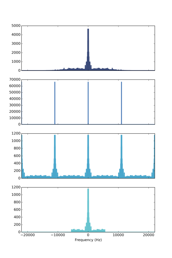
But the result is not very good because

1) We've lost all of the components of the original wave above 5500 Hz, which is the folding frequency of the downsampled wave.

2) Even the components below 5500 Hz are not right, because they still include contributions from the overlapping copies we just clobbered.

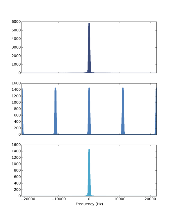
But if we do the same thing again with a bandwidth-limited signal, things are much better:

To understand how we were able to recover the original signal, even after we threw away 75% of the data, we can look more closely at the filter we used to clobber the unwanted copies of the spectrum.  I used a "brick wall" low-pass filter, which has the shape of a boxcar.  And as I showed in a previous chapter, the Fourier transform of a boxcar function is a sinc.  In this example, the window that corresponds to the filter looks like this:

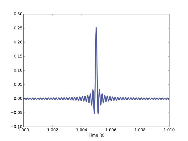
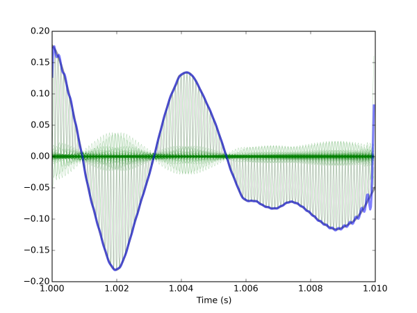
If we zoom in on a shorter segment, we can see more clearly how the interpolation works:

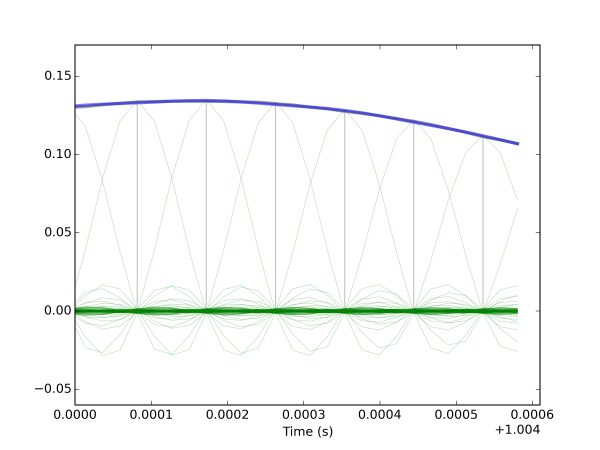
Each sinc function has a peak at the location of one sample and the value 0 at every other sample location.  That way, when we add them up, the sum passes through each of the samples.  In between the samples, the sincs add up to the values of the original signal.

The sampling theorem

In summary, sampling a wave makes copies of its spectrum.  The distance between the copies is the sampling frequency.  If the wave contains components that exceed half of the sampling frequency, the copied spectrums overlap and distort each other.  And when we filter away the unwanted copies, we lose information.

But if the original wave contains no components that exceed half of the sampling frequency, the copies don't overlap, the filter loses no information, and we can recover the original wave exactly.

And that is the Nyquist-Shannon sampling theorem.  Now you should go watch this amazing video that demonstrates the sampling theorem using an analog-to-digital-to-analog converted and two oscilloscopes.

Sign in