Optimizing the Half-band Filters in Multistage Decimation and Interpolation

This blog discusses a not so well-known rule regarding the filtering in multistage decimation and interpolation by an integer power of two. I'm referring to sample rate change systems using half-band lowpass filters (LPFs) as shown in Figure 1. Here's the story.

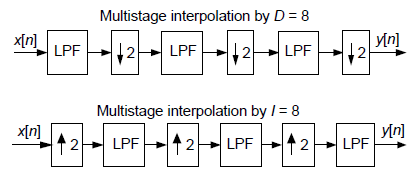
Figure 1: Multistage decimation and interpolation using
half-band filters.

Multistage Decimation – A Very Brief Review

Figure 2(a) depicts the process of decimation by an integer factor D. That is, lowpass FIR (linear-phase) filtering followed by downsampling. The downsampling operation '↓D' means discard all but every Dth input sample.

When the desired decimation factor D is large, say D > 10, a large number of multipliers is necessary within the tapped-delay line of lowpass filter LPF₀. Early DSP pioneers, upon whose shoulders we stand, determined that a more computationally efficient scheme uses multiple decimation stages as shown in Figure 2(b). There the product of integers D₁ and D₂ is our desired overall decimation factor, that is, D₁D₂ = D. The point is, in Figure 2 the sum of the number of multipliers in filters LPF₁ and LPF₂ will be significantly less than the number of multipliers in LPF₀.

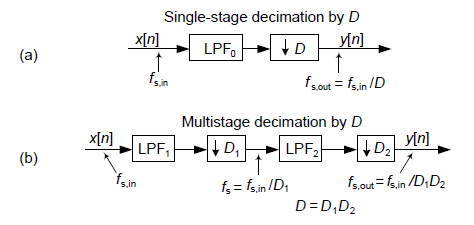
Figure 2: Decimation by integer factor D: (a) single-stage;
(b) multistage.

And, happily, in real-time operations the LPF₂ filter operates at a lower clock rate than the LPF₀ filter. So for decimation by D = 10, the smart thing to do is use the Figure 2(b) implementation where D₁ = 2 and D₂ = 5. Let's now look at multistage decimation by an integer power of two.

Multistage Decimation by an Integer Power of Two

The first focus of this blog is multistage decimation by an integer power of two, such as the decimation by D = 8 process shown in Figure 3. The h_n[k] variables in that figure represent the coefficients of the lowpass FIR filters.

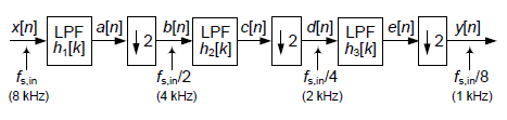
Figure 3: Three-stage decimation by D = 8 using half-band
lowpass filters. Filter impulse responses are h_n[k].

Multistage decimation by an integer power of two is super efficient because all the filters are half-band lowpass filters, where roughly every other filter coefficient is zero-valued. (For example, a 31-tap half-band filter will have only 17 nonzero-valued coefficients).

Years ago when I first saw Figure 3 I thought, "Neat. All I have to do is pass my input signal through a cascade of three identical 'half-band filter and downsample by two' stages." That is, it seemed convenient to use the same half-band filter for each of the three stages. As was pointed out to me, that would be a mistake! [1,2]

As it turns out, the number of h₁[k] coefficients can be less than the number of h₂[k] coefficients. And the number of h₂[k] coefficients can be less than the number of h₃[k] coefficients.

We prove this important principle by way of example starting with Figure 4. That figure shows the spectra of the outputs of the initial operations in Figure 3 when f_s,in = 8 kHz. Figure 4(a) shows the spectrum of our x[n] input signal and the dashed lines in Figure 4(b) show the frequency magnitude response, |H₁(f)|, of our first half-band filter. Figure 4(c) shows that filter's |A(f)| output spectrum.

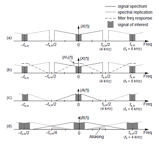
Figure 4: Initial Figure 3 decimation by D = 8 processing:
output spectra.

Figure 4(d) shows that after our first downsample by two operation aliasing does occur. However, that aliased spectral energy (which does not contaminate the spectrum of our dark-shaded signal of interest) will be eliminated in the follow on filtering. Figure 5 shows the spectra of the outputs of the remaining operations in Figure 3.

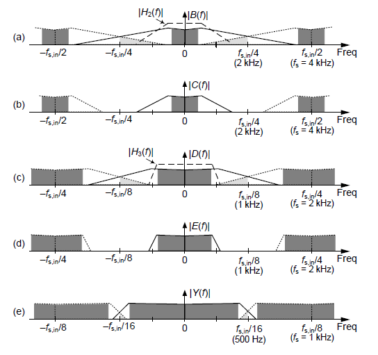
Figure 5: Final Figure 3 decimation by D = 8 processing:
output spectra.

We see in Figures 3 and 4 that the normalized transition region widths, the dashed lines of |H₁(f)|, |H₂(f)|, and |H₃(f)|, of the three half-band filters are different. The transition region widths of the h₁[k] and h₂[k] filters need not be as narrow as the transition region width of the h₃[k] filter. And if the numbers of multipliers in the Figure 3 filters are N₁, N₂, and N₃, we can say:

     For decimation: N₁ < N₂ < N₃.

Thus in our relentless pursuit of computational efficiency, for optimum multistage decimation those three half-band filters will each have a different number of multipliers. That situation is the main point I wanted to make in this blog. Let's conclude this blog by taking a quick look at multistage interpolation by an integer power of two.

Multistage Interpolation by an Integer Power of Two

Figure 6 depicts multistage interpolation by the factor I = 8. An upsampling operation '↑2' means insert one zero-valued sample between each of the upsampler's input samples. The lowpass filters in Figure 6 are linear-phase, symmetrical-coefficient, half-band filters.

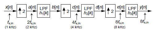
Figure 6: Three-stage interpolation by I = 8 using
half-band lowpass filters

Similar to the multistage decimation in Figure 3, the most efficient implementation of Figure 6's multistage interpolation is to use three different half-band filters. That is, in Figure 6 the number of h₃[k] coefficients can be less than the number of h₂[k] coefficients. And the number of h₂[k] coefficients can be less than the number of h₁[k] coefficients.

We show this situation by way of example starting with Figure 7. That figure shows the spectra of the outputs of the initial operations in Figure 6 when f_s,in = 1000 Hz. Figure 7(a) shows the spectrum of our x[n] input signal. Figure 7(b) shows the spectrum of Figure 6's upsampled by 2 a[n] sequence. The shaded spectral components in Figure 7(b) are the spectral images generated by our first upsampling by two operation. An explanation of why those images exist is given in reference [3].

The dashed lines in Figure 7(b) show the frequency magnitude response, |H₁(f)|, of our first half-band filter whose function is to eliminate the unwanted shaded spectral images in |A(f)|.

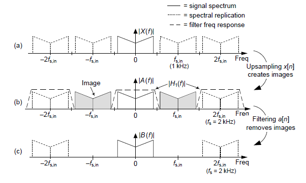
Figure 7: Initial three-stage interpolation by I = 8 processing:
output spectra.

Figure 7(c) shows that filter's |A(f)| output spectrum. Figure 8 shows the output spectra of the four remaining operations in Figure 6.

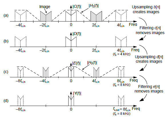
Figure 8: Final three-stage interpolation by I = 8 processing:
output spectra.

By careful examination of the frequency axis values, we can see in Figures 7 and 8 that the normalized transition region widths, the dashed lines of |H₁(f)|, |H₂(f)|, and |H₃(f)|, of the three half-band filters are different. The transition region widths of the h₂[k] and h₃[k] filters need not be as narrow as the transition region width of the h₁[k] filter. Thus if the numbers of multipliers in the Figure 6 filters are N₁, N₂, and N₃, we can say:

     For interpolation: N₁ > N₂ > N₃.

Conclusion

I have shown that multistage sample rate change by an integer power of two is most computationally efficient when the half-band filters each have a different number of multipliers. To quote Forrest Gump, "And that's all I have to say about that."

References

[1] Evgeny Filatov. Private communication. Dec. 20, 2014.
[2] Wolfram Humann. Private communication. Dec. 18, 2015.
[3] http://www.dsprelated.com/showarticle/761.php

Sign in