Signal fitting with subsample resolution

Update: The most recent version can be found here and a demonstration here.
The downloadable code is a "real-life" implementation that is a good choice for "real-life problems", but has grown to almost 700 lines. The code below implements the main functionality only, but is shorter.

Determines sub-sample delay and scaling factor between two signals and resamples / scales one signal to match the other.

For example in measurement automation, it is rather common to apply a test signal to a device-under-test and record the output. A delay is caused both from the latency of measurement instruments and the group delay of the device-under-test itself. In some applications, for example when analyzing the distortion properties of power amplifiers, it is necessary to align the signals within a small fraction of a sample length to avoid systematic errors.

The function fitSignalFFT() determines the delay with sub-sample resolution. It provides a delayed-and-scaled version of one signal that matches the other one.

This code snippet provides an extended version of the implementation in my "delay estimation by FFT" blog entry.

Resampling a signal with a fractional (subsample) delay assumes reconstruction and resampling of an equivalent continuous-time waveform. There are a few "gotchas" such as "ringing" related to the underlying assumptions (cyclic signal, ideal lowpass as reconstruction filter). Some related background can be found in this code snippet (resampling on a regular grid via FFT) and here (resampling at arbitrary time instants by direct evaluation of the Fourier series).

For non-periodic signals, use adequate zero-padding.

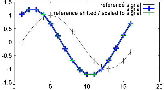
The picture shows an example run:
Two sine waves with different phase and amplitude are used as inputs. The function call returns an offset in samples and a scaling factor that maps the reference signal least-squares-optimally to the other signal.

Further, a delayed and scaled version of the reference signal is returned (green trace, overlapping the blue trace).

Below the example invocation.

ph = (0:15) * 2 * pi / 16;
ref = sin(ph);
sig = 1.23456 * sin(ph + 0.98765)
[coeff, shiftedRef, delta] = fitSignal_FFT(sig, ref);
figure(); hold on;
plot(ref, 'k+-');
h = plot(sig, 'b+-'); set(h, 'lineWidth', 5);
plot(shiftedRef, 'g+-')
legend('reference signal', 'signal', 'reference shifted / scaled to signal');
title('fitSignal\_FFT demo');

Copy the following code snippet into a file fitSignal_FFT.m.