


Spectrum analyzer
Determines the power spectrum, similar to a hardware measurement instrument
The function takes an input signal and gives the two-sided power spectrum. Results are similar to what is obtained using a hardware instrument, when the complex-valued input signal is a baseband-equivalent of a radio frequency signal.
Details can be found from the included examples.
Some highlights:
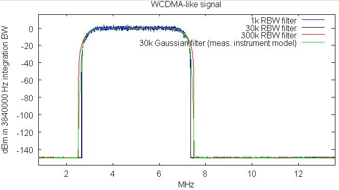
- A resolution bandwidth filter models spectrum measurement by sweeping a bandpass filter and power measurement. Usually the "brickwall" type (ideal bandpass) is the best choice, but also a Gaussian type is implemented.
- The signal's power density is scaled to a user-specified bandwidth. For example, for a WCDMA signal that has a noise bandwidth of 3.84 MHz, the integration bandwidth RBW_power_Hz should be set to 3.84e6, and the power can be read off directly from the trace without further conversion.
- a single-FFT-bin mode is available for discrete-frequency signals (sine waves with an integer number of cycles in the input signal)
- combined averaging and peak detection to make the number of plotted points manageable
- log-scale averaging for logarithmic plots reduces display noise at high frequencies
The included example applies a root-raised cosine filter to a noise signal and plots the spectrum. Since the signal is cyclic, no windowing is necessary. The artificial noisefloor suppresses details below the -150 dBm line.
The second example shows the response of a continuous-time (Laplace-domain) filter on a noise signal and a test pulse.
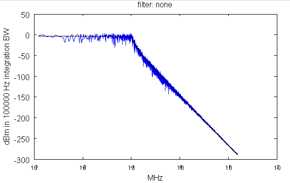
The blue trace is the spectrum of a filtered noise signal, and the black trace results from filtering a test impulse with equal power at all frequencies.
Zooming in reveals that the spectrum analyzer reproduces the frequency response at low offsets accurately, while reducing the amount of data points at higher frequency offsets:
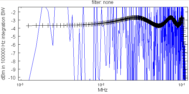
For non-periodic signals, conventional windowing should be applied before calling spectrumAnalyzer().
How to run:
Copy to satest.m and call satest from the command line.
The function spectrumAnalyzer and the helper functions that follow could be copied into an own file spectrumAnalyzer.m.
% ************************************
% spectrum analyzer
% Markus Nentwig, 10.12.2011
%
% Note: If the signal is not cyclic, apply conventional windowing before
% calling spectrumAnalyzer
% ************************************

function satest()
    close all;
    rate_Hz = 30.72e6; % sampling rate
    n = 100000; % number of samples

    noise = randn(1, n);
    pulse = zeros(1, n); pulse(1) = 1;

    % ************************************
    % example (linear frequency scale, RBW filter)
    % ************************************
    tmp1 = normalize(RRC_filter('signal', noise, 'rate_Hz', rate_Hz, 'alpha', 0.22, 'BW_Hz', 3.84e6, 'fCenter_Hz', 5e6));

    % pRef = 0.001: a normalized signal will show as 0 dBm = 0.001 W
    saPar = struct('rate_Hz', rate_Hz, 'fig', 1, 'pRef_W', 1e-3, 'RBW_power_Hz', 3.84e6, 'filter', 'brickwall', 'plotStyle', 'b-');
    spectrumAnalyzer(saPar, 'signal', tmp1, 'RBW_window_Hz', 1e3);
    spectrumAnalyzer(saPar, 'signal', tmp1, 'RBW_window_Hz', 30e3, 'plotStyle', 'k-');
    spectrumAnalyzer(saPar, 'signal', tmp1, 'RBW_window_Hz', 300e3, 'plotStyle', 'r-');
    spectrumAnalyzer(saPar, 'signal', tmp1, 'RBW_window_Hz', 30e3, 'filter', 'gaussian', 'plotStyle', 'g-');
    legend('1k RBW filter', '30k RBW filter', '300k RBW filter', '30k Gaussian filter (meas. instrument model)');
    title('WCDMA-like signal');

    % ************************************
    % example (logarithmic frequency scale,
    % no RBW filter)
    % ************************************
    fPar = struct('rate_Hz', rate_Hz, ...
                  'chebyOrder', 6, ...
                  'chebyRipple_dB', 1, ...
                  'fCorner_Hz', 1e5);

    saPar = struct('rate_Hz', rate_Hz, ...
                   'pRef_W', 1e-3, ...
                   'fMin_Hz', 1e3, ...
                   'RBW_power_Hz', 1e5, ...
                   'RBW_window_Hz', 1e3, ...
                   'filter', 'none', ...
                   'plotStyle', 'b-', ...
                   'logscale', true, ...
                   'fig', 2, ...
                   'noisefloor_dB', -300);

    tmp1 = normalize(IIR_filterExample('signal', noise, fPar));
    tmp2 = normalize(IIR_filterExample('signal', pulse, fPar));

    spectrumAnalyzer('signal', tmp1, saPar);
    spectrumAnalyzer('signal', tmp2, saPar, 'plotStyle', 'k-');
end

function sig = normalize(sig)
    sig = sig / sqrt(sig * sig' / numel(sig));
end

% ************************************
% calculates the frequency that corresponds to each
% FFT bin (negative, zero, positive)
% ************************************
function fb_Hz = FFT_frequencyBasis(n, rate_Hz)
    fb = 0:(n - 1);
    fb = fb + floor(n / 2);
    fb = mod(fb, n);
    fb = fb - floor(n / 2);
    fb = fb / n; % now [0..0.5[, [-0.5..0[
    fb_Hz = fb * rate_Hz;
end

% ************************************
% root-raised cosine filter (to generate
% example signal)
% ************************************
function sig = RRC_filter(varargin)
    def = struct('fCenter_Hz', 0);
    p = vararginToStruct(def, varargin);

    n = numel(p.signal);
    fb_Hz = FFT_frequencyBasis(n, p.rate_Hz);

    % frequency relative to cutoff frequency
    c = abs((fb_Hz - p.fCenter_Hz) / (p.BW_Hz / 2));
    % c=-1 for lower end of transition region
    % c=1 for upper end of transition region
    c=(c-1) / p.alpha;

    % clip to -1..1 range
    c=min(c, 1);
    c=max(c, -1);

    % raised-cosine filter
    H = 1/2+cos(pi/2*(c+1))/2;

    % root-raised cosine filter
    H = sqrt(H);

    % apply filter
    sig = ifft(fft(p.signal) .* H);
end

% ************************************
% continuous-time filter example
% ************************************
function sig = IIR_filterExample(varargin)
    p = vararginToStruct(varargin);

    % design continuous-time IIR filter
    [IIR_b, IIR_a] = cheby1(p.chebyOrder, p.chebyRipple_dB, 1, 's');

    % evaluate on the FFT frequency grid
    fb_Hz = FFT_frequencyBasis(numel(p.signal), p.rate_Hz);

    % Laplace domain operator, normalized to filter cutoff frequency
    % (the above cheby1 call designs for unity cutoff)
    s = 1i * fb_Hz / p.fCorner_Hz;

    % polynomial in s
    H_num = polyval(IIR_b, s);
    H_denom = polyval(IIR_a, s);
    H = H_num ./ H_denom;

    % apply filter
    sig = ifft(fft(p.signal) .* H);
end

% ----------------------------------------------------------------------
% optionally: Move the code below into spectrumAnalyzer.m
function [fr, fb, handle] = spectrumAnalyzer(varargin)
    def = struct(...
        'noisefloor_dB', -150, ...
        'filter', 'none', ...
        'logscale', false,  ...
        'NMax', 10000, ...
        'freqUnit', 'MHz', ...
        'fig', -1, ...
        'plotStyle', 'b-', ...
        'originMapsTo_Hz', 0 ...
        );

    p = vararginToStruct(def, varargin);
    signal = p.signal;

    handle=nan; % avoid warning

    % A resolution bandwidth value of 'sine' sets the RBW to the FFT bin spacing.
    % The power of a pure sine wave now shows correctly from the peak in the spectrum (unity => 0 dB)
    singleBinMode=strcmp(p.RBW_power_Hz, 'sine');

    nSamples = numel(p.signal);
    binspacing_Hz = p.rate_Hz / nSamples;
    windowBW=p.RBW_window_Hz;
    noisefloor=10^(p.noisefloor_dB/10);
    % factor in the scaling factor that will be applied later for conversion to
    % power in RBW
    if ~singleBinMode
        noisefloor = noisefloor * binspacing_Hz / p.RBW_power_Hz;
    end

    % fr: "f"requency "r"esponse (plot y data)
    % fb: "f"requency "b"ase (plot x data)
    fr = fft(p.signal);

    scale_to_dBm=sqrt(p.pRef_W/0.001);

    % Normalize amplitude to the number of samples that contribute
    % to the spectrum
    fr=fr*scale_to_dBm/nSamples;

    % magnitude
    fr = fr .* conj(fr);

    [winLeft, winRight] = spectrumAnalyzerGetWindow(p.filter, singleBinMode, p.RBW_window_Hz, binspacing_Hz);
    % winLeft is the right half of the window, but it appears on the
    % left side of the FFT space

    winLen=0;
    if ~isempty(winLeft)

        % zero-pad the power spectrum in the middle with a length
        % equivalent to the window size.
        % this guarantees that there is enough bandwidth for the filter!
        % one window length is enough, the spillover from both sides overlaps
        % Scale accordingly.
        winLen=size(winLeft, 2)+size(winRight, 2);

        % note: fr is the power shown in the plot, NOT a frequency
        % domain representation of a signal.
        % There is no need to renormalize because of the length change
        center=floor(nSamples/2)+1;
        rem=nSamples-center;
        fr=[fr(1:center-1), zeros(1, winLen-1), fr(center:end)];
        % construct window with same length as fr
        win=zeros(size(fr));
        win(1:1+size(winLeft, 2)-1)=winLeft;
        win(end-size(winRight, 2)+1:end)=winRight;

        assert(isreal(win));
        assert(isreal(fr));
        assert(size(win, 2)==size(fr, 2));

        % convolve using FFT
        win=fft(win);
        fr=fft(fr);

        fr=fr .* win;
        fr=ifft(fr);
        fr=real(fr); % chop off roundoff error imaginary part
        fr=max(fr, 0); % chop off small negative numbers

        % remove padding
        fr=[fr(1:center-1), fr(end-rem+1:end)];
    end

    % ************************************
    % build frequency basis and rotate 0 Hz to center
    % ************************************
    fb = FFT_frequencyBasis(numel(fr), p.rate_Hz);
    fr = fftshift(fr);
    fb = fftshift(fb);

    if false
        % use in special cases (very long signals)

        % ************************************
        % data reduction:
        % If a filter is used, details smaller than windowBW are
        % suppressed already by the filter, and using more samples
        % gives no additional information.
        % ************************************
        if numel(fr) > p.NMax
            switch(p.filter)
              case 'gaussian'
                % 0.2 offset from the peak causes about 0.12 dB error
                incr=floor(windowBW/binspacing_Hz/5);
              case 'brickwall'
                % there is no error at all for a peak
                incr=floor(windowBW/binspacing_Hz/3);
              case 'none'
                % there is no filter, we cannot discard data at this stage
                incr=-1;
            end

            if incr > 1
                fr=fr(1:incr:end);
                fb=fb(1:incr:end);
            end
        end
    end

    % ************************************
    % data reduction:
    % discard beyond fMin / fMax, if given
    % ************************************
    indexMin = 1;
    indexMax = numel(fb);
    flag=0;
    if isfield(p, 'fMin_Hz')
        indexMin=min(find(fb >= p.fMin_Hz));
        flag=1;
    end
    if isfield(p, 'fMax_Hz')
        indexMax=max(find(fb <= p.fMax_Hz));
        flag=1;
    end
    if flag
        fb=fb(indexMin:indexMax);
        fr=fr(indexMin:indexMax);
    end

    if p.NMax > 0
        if p.logscale
            % ************************************
            % Sample number reduction for logarithmic
            % frequency scale
            % ************************************
            assert(isfield(p, 'fMin_Hz'), 'need fMin_Hz in logscale mode');
            assert(p.fMin_Hz > 0, 'need fMin_Hz > 0 in logscale mode');
            if ~isfield(p, 'fMax_Hz')
                p.fMax_Hz = p.rate_Hz / 2;
            end

            % averaged output arrays
            fbOut=zeros(1, p.NMax-1);
            frOut=zeros(1, p.NMax-1);

            % candidate output frequencies (it's not certain yet
            % that there is actually data)
            s=logspace(log10(p.fMin_Hz), log10(p.fMax_Hz), p.NMax);

            f1=s(1);
            nextStartIndex=max(find(fb < f1));
            if isempty(nextStartIndex)
                nextStartIndex=1;
            end

            % iterate through all frequency regions
            % collect data
            % average
            for index=2:size(s, 2)
                f2=s(index);
                endIndex=max(find(fb < f2));

                % number of data points in bin
                n=endIndex-nextStartIndex+1;
                if n > 0
                    % average
                    ix=nextStartIndex:endIndex;
                    fbOut(index-1)=sum(fb(ix))/n;
                    frOut(index-1)=sum(fr(ix))/n;
                    nextStartIndex=endIndex+1;
                else
                    % mark point as invalid (no data)
                    fbOut(index-1)=nan;
                end
            end
            % remove bins where no data point contributed
            ix=find(~isnan(fbOut));
            fbOut=fbOut(ix);
            frOut=frOut(ix);
            fb=fbOut;
            fr=frOut;
        else
            % ************************************
            % Sample number reduction for linear
            % frequency scale
            % ************************************
            len=size(fb, 2);
            decim=ceil(len/p.NMax); % one sample overlength => decim=2
            if decim > 1
                % truncate to integer multiple
                len=floor(len / decim)*decim;
                fr=fr(1:len);
                fb=fb(1:len);

                fr=reshape(fr, [decim, len/decim]);
                fb=reshape(fb, [decim, len/decim]);
                if singleBinMode
                    % apply peak hold over each segment (column)
                    fr=max(fr);
                else
                    % apply averaging over each segment (column)
                    fr = sum(fr) / decim;
                end
                fb=sum(fb)/decim; % for each column the average
            end % if sample reduction necessary
        end % if linear scale
    end % if sample number reduction

    % ************************************
    % convert magnitude to dB.
    % truncate very small values
    % using an artificial noise floor
    % ************************************
    fr=(10*log10(fr+noisefloor));

    if singleBinMode
        % ************************************
        % The power reading shows the content of each
        % FFT bin. This is accurate for single-frequency
        % tones that fall exactly on the frequency grid
        % (an integer number of cycles over the signal length)
        % ************************************
    else
        % ************************************
        % convert sensed power density from FFT bin spacing
        % to resolution bandwidth
        % ************************************
        fr=fr+10*log10(p.RBW_power_Hz/binspacing_Hz);
    end

    % ************************************
    % Post-processing:
    % Translate frequency axis to RF
    % ************************************
    fb = fb + p.originMapsTo_Hz;

    % ************************************
    % convert to requested units
    % ************************************
    switch(p.freqUnit)
      case 'Hz'
      case 'kHz'
        fb = fb / 1e3;
      case 'MHz'
        fb = fb / 1e6;
      case 'GHz'
        fb = fb / 1e9;
      otherwise
        error('unsupported frequency unit');
    end

    % ************************************
    % Plot (if requested)
    % ************************************
    if p.fig > 0
        % *************************************************************
        % title
        % *************************************************************
        if isfield(p, 'title')
            t=['"', p.title, '";'];
        else
            t='';
        end
        switch(p.filter)
          case 'gaussian'
            t=[t, ' filter: Gaussian '];
          case 'brickwall'
            t=[t, ' filter: ideal bandpass '];
          case 'none'
            t=[t, ' filter: none '];
          otherwise
            assert(0)
        end

        if ~strcmp(p.filter, 'none')
            t=[t, '(', mat2str(p.RBW_window_Hz), ' Hz)'];
        end

        if isfield(p, 'pNom_dBm')
            % *************************************************************
            % show dB relative to a given absolute power in dBm
            % *************************************************************
            fr=fr-p.pNom_dBm;
            yUnit='dB';
        else
            yUnit='dBm';
        end

        % *************************************************************
        % plot
        % *************************************************************
        figure(p.fig);
        if p.logscale
            handle = semilogx(fb, fr, p.plotStyle);
        else
            handle = plot(fb, fr, p.plotStyle);
        end
        hold on; % after plot, otherwise prevents logscale

        if isfield(p, 'lineWidth')
            set(handle, 'lineWidth', p.lineWidth);
        end

        % *************************************************************
        % axis labels
        % *************************************************************
        xlabel(p.freqUnit);
        if singleBinMode
            ylabel([yUnit, ' (continuous wave)']);
        else
            ylabel([yUnit, ' in ', mat2str(p.RBW_power_Hz), ' Hz integration BW']);
        end
        title(t);

        % *************************************************************
        % adapt y range, if requested
        % *************************************************************
        y=ylim();
        y1=y(1); y2=y(2);

        rescale=false;
        if isfield(p, 'yMin')
            y(1)=p.yMin;
            rescale=true;
        end
        if isfield(p, 'yMax')
            y(2)=p.yMax;
            rescale=true;
        end
        if rescale
            ylim(y);
        end
    end
end

function [winLeft, winRight] = spectrumAnalyzerGetWindow(filter, singleBinMode, RBW_window_Hz, binspacing_Hz)

    switch(filter)
      case 'gaussian'

        % construct Gaussian filter
        % -60 / -3 dB shape factor 4.472
        nRBW=6;
        nOneSide=ceil(RBW_window_Hz/binspacing_Hz*nRBW);

        filterBase=linspace(0, nRBW, nOneSide);
        winLeft=exp(-(filterBase*0.831) .^2);
        winRight=fliplr(winLeft(2:end)); % omit 0 Hz bin

      case 'brickwall'
        nRBW=1;
        n=ceil(RBW_window_Hz/binspacing_Hz*nRBW);
        n1 = floor(n/2);
        n2 = n - n1;

        winLeft=ones(1, n1);
        winRight=ones(1, n2);

      case 'none'
        winLeft=[];
        winRight=[];

      otherwise
        error('unknown RBW filter type');
    end

    % the window is not supposed to shift the spectrum.
    % Therefore, the first bin is always in winLeft (0 Hz):
    if size(winLeft, 2)==1 && isempty(winRight)
        % there is no use to convolve with one-sample window
        % it's always unity
        winLeft=[];
        winRight=[];
        tmpwin=[];
    end

    if ~isempty(winLeft)
        % (note: it is not possible that winRight is empty, while winLeft is not)
        if singleBinMode
            % normalize to unity at 0 Hz
            s=winLeft(1);
        else
            % normalize to unity area under the filter
            s=sum(winLeft)+sum(winRight);
        end
        winLeft=winLeft / s;
        winRight=winRight / s;
    end
end

% *************************************************************
% helper function: Parse varargin argument list
% allows calling myFunc(A, A, A, ...)
% where A is
% - key (string), value (arbitrary) => result.key = value
% - a struct => fields of A are copied to result
% - a cell array => recursive handling using above rules
% *************************************************************
function r = vararginToStruct(varargin)
% note: use of varargin implicitly packs the caller's arguments into a cell array
% that is, calling vararginToStruct('hello') results in
%   varargin = {'hello'}
    r = flattenCellArray(varargin, struct());
end

function r = flattenCellArray(arr, r)
    ix=1;
    ixMax = numel(arr);
    while ix <= ixMax
        e = arr{ix};

        if iscell(e)
            % cell array at 'key' position gets recursively flattened
            % becomes struct
            r = flattenCellArray(e, r);
        elseif ischar(e)
            % string => key.
            % The following entry is a value
            ix = ix + 1;
            v = arr{ix};
            % store key-value pair
            r.(e) = v;
        elseif isstruct(e)
            names = fieldnames(e);
            for ix2 = 1:numel(names)
                k = names{ix2};
                r.(k) = e.(k);
            end
        else
            e
            assert(false)
        end
        ix=ix+1;
    end % while
end


