


Alias/error simulation of interpolating RRC filter
Shows alias and error spectrum of a root-raised cosine/upsample-by-64 multi-stage polyphase FIR.
Documentation:
Data files (impulse responses):
Included in the zip archive.
Example output
Description
In some types of radio transmitters (for example WCDMA), the symbol stream is processed with a pulse-shaping filter and upsampled to a higher rate for digital-to-analog conversion. It is impractical to perform both pulse-shaping and sample-rate conversion in a single step (an equivalent FIR filter would require about 2500 coefficients and 20 multiply-accumulate operations per output sample). The example design implements first pulse-shaping at an oversampling factor of 2, and then sample rate conversion by factors of 2, 2 and 4.
The spectrum of the input signal is known, the frequency locations of all alias products at every filtering stage can be predicted, and stopband attenuation needs to be implemented only at alias frequencies.
The purpose of this code snippet is to evaluate both the alias response and the in-channel distortion to compare performance against requirements.
The design scripts for the individual filter stages are also included.
Download
The zip archive contains
- eval_RRC_resampler.m: The code snippet
- RRC.dat: A root-raised cosine polyphase FIR filter at output rate 2 (32 taps, 64 coefficients)
- ip1.dat: A polyphase interpolator at output rate 4 (7 taps, 14 coefficients)
- ip2.dat: A polyphase interpolator at output rate 8 (4 taps, 8 coefficients)
- ip3.dat: A polyphase interpolator at output rate 16 (3 taps, 6 coefficients)
- ip4.dat: A polyphase interpolator at output rate 64 (2 taps, 8 coefficients)
- design_RRC.m: Filter design script for RRC, writes RRC.dat
- design_ip1.m: Filter design script for ip1, writes ip1.dat
- design_ip2.m: Filter design script for ip2, writes ip2.dat
- design_ip3.m: Filter design script for ip3, writes ip3. dat
- design_ip4.m: Filter design script for ip4, writes ip4.dat
- @YAFIR folder: filter design library (Description here. Note that the included version is slightly extended, compared to the single-file code snippet)
How to run
- Download the zip archive and unpack to a folder.
- "cd" into the folder from the Matlab / Octave command line.
- Run eval_RRC_resampler.
- Edit and run a filter design script (overwrites impulse response)
- Re-run eval_RRC_resampler to observe changes in the total response.
Equalized filter
There is also an option for an alternative, equalized RRC filter that compensates for non-idealities of the sample rate conversion. It achieves considerably lower vector error at the "worst" frequencies.
Equalization in the RRC filter is more efficient than improving the resampler, since manipulations on the passband frequency response are implemented most easily at the lowest possible sampling rate.
The corresponding "smode=xyz" lines are commented out by default:
- eval_RRC_resampler with smode="evalIdeal" evaluates and writes the resampler frequency response as "InterpolatorFrequencyResponse.mat"
- design_RRC_filter with smode="equalized" designs an equalized RRC filter as "RRC_equalized.dat"
- running eval_RRC_resampler a second time with mode="evalEqualized" evaluates the design with the equalized RRC filter.
Comments
Sample rate conversion with FIR filters is straightforward to design, but not necessarily the most efficient approach. Especially for the last stages, the FIR filtering gets surprisingly "expensive" (in terms of MAC operations per output sample) due to the high sampling rate. Alternative methods (IIR/CIC etc) are well known.
A modified resampler should be designed mainly for alias rejection. Then use the RRC filter to equalize a non-ideal passband response, as shown in the example files.
% *************************************************
% alias- and in-channel error analysis for root-raised
% cosine filter with upsampler FIR cascade
% Markus Nentwig, 25.12.2011
%
% * plots the aliases at the output of each stage
% * plots the error spectrum (deviation from ideal RRC-
% response)
% *************************************************
function eval_RRC_resampler()
1;
% variant 1
% conventional RRC filter and FIR resampler
smode = 'evalConventional';
% export resampler frequency response to design equalizing RRC filter
%smode = 'evalIdeal';
% variant 2
% equalizing RRC filter and FIR resampler
% smode = 'evalEqualized';
% *************************************************
% load impulse responses
% *************************************************
switch smode
case 'evalConventional'
% conventionally designed RRC filter
h0 = load('RRC.dat');
case 'evalIdeal'
h0 = 1;
case 'evalEqualized'
% alternative RRC design that equalizes the known frequency
% response of the resampler
h0 = load('RRC_equalized.dat');
otherwise assert(false);
end
h1 = load('ip1.dat');
h2 = load('ip2.dat');
h3 = load('ip3.dat');
h4 = load('ip4.dat');
% *************************************************
% --- signal source ---
% *************************************************
n = 10000; % test signal, number of symbol lengths
rate = 1;
s = zeros(1, n);
s(1) = 1;
p = {};
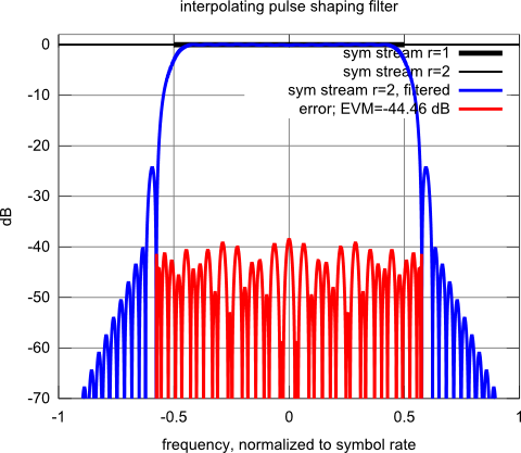
p = addPlot(p, s, rate, 'k', 5, 'sym stream r=1');
% *************************************************
% --- upsampling RRC filter ---
% *************************************************
rate = rate * 2;
s = upsample(s, 2); % insert one zero after every sample
p = addPlot(p, s, rate, 'k', 2, 'sym stream r=2');
s = filter(h0, [1], s);
p = addPlot(p, s, rate, 'b', 3, 'sym stream r=2, filtered');
p = addErrPlot(p, s, rate, 'error');
figure(1); clf; grid on; hold on;
doplot(p, 'interpolating pulse shaping filter');
ylim([-70, 2]);
p = {};
% *************************************************
% --- first interpolator by 2 ---
% *************************************************
rate = rate * 2;
s = upsample(s, 2); % insert one zero after every sample
p = addPlot(p, s, rate, 'k', 3, 'interpolator 1 input');
s = filter(h1, [1], s);
p = addPlot(p, s, rate, 'b', 3, 'interpolator 1 output');
p = addErrPlot(p, s, rate, 'error');
figure(2); clf; grid on; hold on;
doplot(p, 'first interpolator by 2');
ylim([-70, 2]);
p = {};
% *************************************************
% --- second interpolator by 2 ---
% *************************************************
rate = rate * 2;
s = upsample(s, 2); % insert one zero after every sample
p = addPlot(p, s, rate, 'k', 3, 'interpolator 2 input');
s = filter(h2, [1], s);
p = addPlot(p, s, rate, 'b', 3, 'interpolator 2 output');
p = addErrPlot(p, s, rate, 'error');
figure(3); clf; grid on; hold on;
doplot(p, 'second interpolator by 2');
ylim([-70, 2]);
p = {};
% *************************************************
% --- third interpolator by 2 ---
% *************************************************
rate = rate * 2;
s = upsample(s, 2); % insert one zero after every sample
p = addPlot(p, s, rate, 'k', 3, 'interpolator 3 input');
s = filter(h3, [1], s);
p = addPlot(p, s, rate, 'b', 3, 'interpolator 3 output');
p = addErrPlot(p, s, rate, 'error');
figure(4); clf; grid on; hold on;
doplot(p, 'third interpolator by 2');
ylim([-70, 2]);
p = {};
% *************************************************
% --- fourth interpolator by 4 ---
% *************************************************
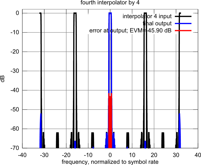
rate = rate * 4;
s = upsample(s, 4); % insert three zeros after every sample
p = addPlot(p, s, rate, 'k', 3, 'interpolator 4 input');
s = filter(h4, [1], s);
p = addPlot(p, s, rate, 'b', 3, 'final output');
p = addErrPlot(p, s, rate, 'error at output');
figure(5); clf; grid on; hold on;
doplot(p, 'fourth interpolator by 4');
ylim([-70, 2]);
figure(334);
stem(real(s(1:10000)));
% *************************************************
% export resampler frequency response
% *************************************************
switch smode
case 'evalIdeal'
exportFrequencyResponse(s, rate, 'interpolatorFrequencyResponse.mat');
end
end
% ************************************
% put frequency response plot data into p
% ************************************
function p = addPlot(p, s, rate, plotstyle, linewidth, legtext)
p{end+1} = struct('sig', s, 'rate', rate, 'plotstyle', plotstyle, 'linewidth', linewidth, 'legtext', legtext);
end
% ************************************
% determine the error spectrum, compared to an ideal filter (RRC)
% and add a plot to p
% ************************************
function p = addErrPlot(p, s, rate, legtext)
ref = RRC_impulseResponse(numel(s), rate);
% refB is scaled and shifted (sub-sample resolution) replica of ref
% that minimizes the energy in (s - refB)
[coeff, refB, deltaN] = fitSignal_FFT(s, ref);
err = s - refB;
err = brickwallFilter(err, rate, 1.15); % 1+alpha
% signal is divided into three parts:
% - A) wanted in-channel energy (correlated with ref)
% - B) unwanted in-channel energy (uncorrelated with ref)
% - C) unwanted out-of-channel energy (aliases)
% the error vector magnitude is B) relative to A)
energySig = refB * refB';
energyErr = err * err';
EVM_dB = 10*log10(energyErr / energySig);
legtext = sprintf('%s; EVM=%1.2f dB', legtext, EVM_dB);
p{end+1} = struct('sig', err, 'rate', rate, 'plotstyle', 'r', 'linewidth', 3, 'legtext', legtext);
end
% ************************************
% helper function, plot data in p
% ************************************
function doplot(p, t)
leg = {};
for ix = 1:numel(p)
pp = p{ix};
fb = FFT_frequencyBasis(numel(pp.sig), pp.rate);
fr = 20*log10(abs(fft(pp.sig) + eps));
h = plot(fftshift(fb), fftshift(fr), pp.plotstyle);
set(h, 'lineWidth', pp.linewidth);
xlabel('frequency, normalized to symbol rate');
ylabel('dB');
leg{end+1} = pp.legtext;
end
legend(leg);
title(t);
end
% ************************************
% ideal RRC filter (impulse response is as
% long as test signal)
% ************************************
function ir = RRC_impulseResponse(n, rate)
alpha = 0.15;
fb = FFT_frequencyBasis(n, rate);
% bandwidth is 1
c = abs(fb / 0.5);
c = (c-1)/(alpha); % -1..1 in the transition region
c=min(c, 1);
c=max(c, -1);
RRC_h = sqrt(1/2+cos(pi/2*(c+1))/2);
ir = real(ifft(RRC_h));
end
% ************************************
% remove any energy at frequencies > BW/2
% ************************************
function s = brickwallFilter(s, rate, BW)
n = numel(s);
fb = FFT_frequencyBasis(n, rate);
ix = find(abs(fb) > BW / 2);
s = fft(s);
s(ix) = 0;
s = real(ifft(s));
end
% ************************************
% for an impulse response s at rate, write the
% frequency response to fname
% ************************************
function exportFrequencyResponse(s, rate, fname)
fb = fftshift(FFT_frequencyBasis(numel(s), rate));
fr = fftshift(fft(s));
figure(335); grid on;
plot(fb, 20*log10(abs(fr)));
title('exported frequency response');
xlabel('normalized frequency');
ylabel('dB');
save(fname, 'fb', 'fr');
end
% ************************************
% calculates the frequency that corresponds to
% each FFT bin (negative, zero, positive)
% ************************************
function fb_Hz = FFT_frequencyBasis(n, rate_Hz)
fb = 0:(n - 1);
fb = fb + floor(n / 2);
fb = mod(fb, n);
fb = fb - floor(n / 2);
fb = fb / n; % now [0..0.5[, [-0.5..0[
fb_Hz = fb * rate_Hz;
end
% *******************************************************
% delay-matching between two signals (complex/real-valued)
%
% * matches the continuous-time equivalent waveforms
% of the signal vectors (reconstruction at Nyquist limit =>
% ideal lowpass filter)
% * Signals are considered cyclic. Use arbitrary-length
% zero-padding to turn a one-shot signal into a cyclic one.
%
% * output:
% => coeff: complex scaling factor that scales 'ref' into 'signal'
% => delay 'deltaN' in units of samples (subsample resolution)
% apply both to minimize the least-square residual
% => 'shiftedRef': a shifted and scaled version of 'ref' that
% matches 'signal'
% => (signal - shiftedRef) gives the residual (vector error)
%
% Example application
% - with a full-duplex soundcard, transmit an arbitrary cyclic test signal 'ref'
% - record 'signal' at the same time
% - extract one arbitrary cycle
% - run fitSignal
% - deltaN gives the delay between both with subsample precision
% - 'shiftedRef' is the reference signal fractionally resampled
% and scaled to optimally match 'signal'
% - to resample 'signal' instead, exchange the input arguments
% *******************************************************
function [coeff, shiftedRef, deltaN] = fitSignal_FFT(signal, ref)
n=length(signal);
% xyz_FD: Frequency Domain
% xyz_TD: Time Domain
% all references to 'time' and 'frequency' are for illustration only
forceReal = isreal(signal) && isreal(ref);
% *******************************************************
% Calculate the frequency that corresponds to each FFT bin
% [-0.5..0.5[
% *******************************************************
binFreq=(mod(((0:n-1)+floor(n/2)), n)-floor(n/2))/n;
% *******************************************************
% Delay calculation starts:
% Convert to frequency domain...
% *******************************************************
sig_FD = fft(signal);
ref_FD = fft(ref, n);
% *******************************************************
% ... calculate crosscorrelation between
% signal and reference...
% *******************************************************
u=sig_FD .* conj(ref_FD);
if mod(n, 2) == 0
% for an even sized FFT the center bin represents a signal
% [-1 1 -1 1 ...] (subject to interpretation). It cannot be delayed.
% The frequency component is therefore excluded from the calculation.
u(length(u)/2+1)=0;
end
Xcor=abs(ifft(u));
% figure(); plot(abs(Xcor));
% *******************************************************
% Each bin in Xcor corresponds to a given delay in samples.
% The bin with the highest absolute value corresponds to
% the delay where maximum correlation occurs.
% *******************************************************
integerDelay = find(Xcor==max(Xcor));
% (1): in case there are several bitwise identical peaks, use the first one
% Minus one: Delay 0 appears in bin 1
integerDelay=integerDelay(1)-1;
% Fourier transform of a pulse shifted by one sample
rotN = exp(2i*pi*integerDelay .* binFreq);
uDelayPhase = -2*pi*binFreq;
% *******************************************************
% Since the signal was multiplied with the conjugate of the
% reference, the phase is rotated back to 0 degrees in case
% of no delay. Delay appears as linear increase in phase, but
% it has discontinuities.
% Use the known phase (with +/- 1/2 sample accuracy) to
% rotate back the phase. This removes the discontinuities.
% *******************************************************
% figure(); plot(angle(u)); title('phase before rotation');
u=u .* rotN;
% figure(); plot(angle(u)); title('phase after rotation');
% *******************************************************
% Obtain the delay using linear least mean squares fit
% The phase is weighted according to the amplitude.
% This suppresses the error caused by frequencies with
% little power, that may have radically different phase.
% *******************************************************
weight = abs(u);
constRotPhase = 1 .* weight;
uDelayPhase = uDelayPhase .* weight;
ang = angle(u) .* weight;
r = [constRotPhase; uDelayPhase] .' \ ang.'; %linear mean square
%rotPhase=r(1); % constant phase rotation, not used.
% the same will be obtained via the phase of 'coeff' further down
fractionalDelay=r(2);
% *******************************************************
% Finally, the total delay is the sum of integer part and
% fractional part.
% *******************************************************
deltaN = integerDelay + fractionalDelay;
% *******************************************************
% provide shifted and scaled 'ref' signal
% *******************************************************
% this is effectively time-convolution with a unit pulse shifted by deltaN
rotN = exp(-2i*pi*deltaN .* binFreq);
ref_FD = ref_FD .* rotN;
shiftedRef = ifft(ref_FD);
% *******************************************************
% Again, crosscorrelation with the now time-aligned signal
% *******************************************************
coeff=sum(signal .* conj(shiftedRef)) / sum(shiftedRef .* conj(shiftedRef));
shiftedRef=shiftedRef * coeff;
if forceReal
shiftedRef = real(shiftedRef);
end
end


