Halfband Filter Design with Python/Scipy

The following code snippet is an example how to design a half band filter.  Half band filters are interesting because every even coefficient, except 0, is 0.  Those multiplications do not need to be performed, additional calculation reduction can be gained by implementing a folded FIR (coeffecients are symmetric).  Only 1/4 the multiplies are required for a straight-forward implementation.  Also, polyphase implementations [1] reduce the required number of multiplications even further.

This code snippet is an example how to design a half band filter using the remez function in the Python scipy.signal package.

A half band filter can be designed using the Parks-McCellen equilripple design methods by having equal offsets of the pass-band and stop-band (from filter specification) and equal weights of the pass-band and stop-band [2].

Filter Specification: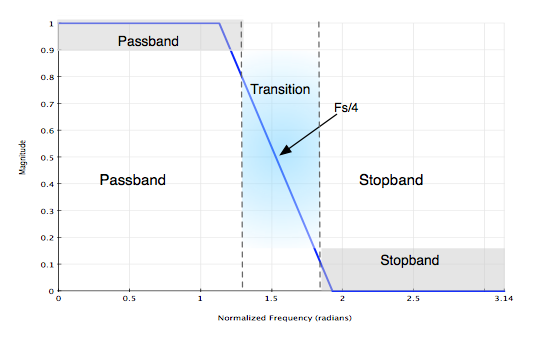



The code snippet below is an iPython session.  The numpy/scipy packages are required.  The "remez" function is part of the scipy.signal package.  The following plot is generated from the code snippet output and shows the filter response, in dB, for the filter length in the example.

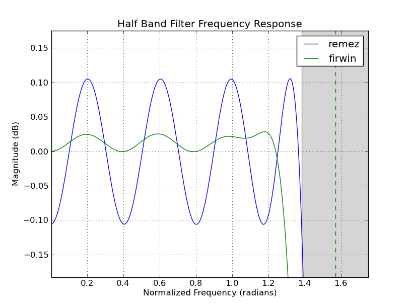
A commentor, @kaz, pointed out that the firwin design produces lower attenuation in the stopband and less ripple in the passband.  But the firwin design has a slower transition band.  In multi-rate systems which use the halfband filter and decimate by 2 more signal beyond Fs/4 will be aliased.  This is a consideration for the designer.  The windowed frequency sampling design (scipy.signal firwin, Matlab fir1) produces the same strucutre, every other coefficient 0 so it can be used in an optimized implementation.

The coefficients from this design are :

          remez       firwin
------------------------------------
 tap  0   0.000000    0.000000
 tap  1  -0.010233   -0.001888
 tap  2   0.000000    0.000000
 tap  3   0.010668    0.003862
 tap  4   0.000000    0.000000
 tap  5  -0.016324   -0.008242
 tap  6   0.000000    0.000000
 tap  7   0.024377    0.015947
 tap  8   0.000000    0.000000
 tap  9  -0.036482   -0.028677
 tap 10   0.000000    0.000000
 tap 11   0.056990    0.050719
 tap 12   0.000000    0.000000
 tap 13  -0.101993   -0.098016
 tap 14   0.000000    0.000000
 tap 15   0.316926    0.315942
 tap 16   0.500009    0.500706
 tap 17   0.316926    0.315942
 tap 18   0.000000    0.000000
 tap 19  -0.101993   -0.098016
 tap 20   0.000000    0.000000
 tap 21   0.056990    0.050719
 tap 22   0.000000    0.000000
 tap 23  -0.036482   -0.028677
 tap 24   0.000000    0.000000
 tap 25   0.024377    0.015947
 tap 26   0.000000    0.000000
 tap 27  -0.016324   -0.008242
 tap 28   0.000000    0.000000
 tap 29   0.010668    0.003862
 tap 30   0.000000    0.000000
 tap 31  -0.010233   -0.001888
 tap 32   0.000000    0.000000   

Every other coeffecient is zero as expected.

[1] Lyons, Rick, "Understanding Digital Signal Processing", 3rd Ed, Pearson 2011
[2] Harris, Fred, "Multirate Signal Processing",  Pearson 2004
[3] McClellan, Parks, "A Personal History of the Parks-McClellan Algorithm", IEEE Signal Processing Magazine 2005.

# The following is a Python/scipy snippet to generate the 
# coefficients for a halfband filter.  A halfband filter
# is a filter where the cutoff frequency is Fs/4 and every
# other coeffecient is zero except the cetner tap.
# Note: every other (even except 0) is 0, most of the coefficients
#       will be close to zero, force to zero actual

import numpy
from numpy import log10, abs, pi
import scipy
from scipy import signal
import matplotlib
import matplotlib.pyplot
import matplotlib as mpl

# ~~[Filter Design with Parks-McClellan Remez]~~
N = 32  # Filter order
# Filter symetric around 0.25 (where .5 is pi or Fs/2)
bands = numpy.array([0., .22, .28, .5])
h = signal.remez(N+1, bands, [1,0], [1,1])
h[abs(h) <= 1e-4] = 0.
(w,H) = signal.freqz(h)

# ~~[Filter Design with Windowed freq]~~
b = signal.firwin(N+1, 0.5)
b[abs(h) <= 1e-4] = 0.
(wb, Hb) = signal.freqz(b)

# Dump the coefficients for comparison and verification
print('          remez       firwin')
print('------------------------------------')
for ii in range(N+1):
    print(' tap %2d   %-3.6f    %-3.6f' % (ii, h[ii], b[ii]))

## ~~[Plotting]~~
# Note: the pylab functions can be used to create plots,
#       and these might be easier for beginners or more familiar
#       for Matlab users.  pylab is a wrapper around lower-level
#       MPL artist (pyplot) functions.
fig = mpl.pyplot.figure()
ax0 = fig.add_subplot(211)
ax0.stem(numpy.arange(len(h)), h)
ax0.grid(True)
ax0.set_title('Parks-McClellan (remez) Impulse Response')
ax1 = fig.add_subplot(212)
ax1.stem(numpy.arange(len(b)), b)
ax1.set_title('Windowed Frequency Sampling (firwin) Impulse Response')
ax1.grid(True)
fig.savefig('hb_imp.png')

fig = mpl.pyplot.figure()
ax1 = fig.add_subplot(111)
ax1.plot(w, 20*log10(abs(H)))
ax1.plot(w, 20*log10(abs(Hb)))
ax1.legend(['remez', 'firwin'])
bx = bands*2*pi
ax1.axvspan(bx[1], bx[2], facecolor='0.5', alpha='0.33')
ax1.plot(pi/2, -6, 'go')
ax1.axvline(pi/2, color='g', linestyle='--')
ax1.axis([0,pi,-64,3])
ax1.grid('on')
ax1.set_ylabel('Magnitude (dB)')
ax1.set_xlabel('Normalized Frequency (radians)')
ax1.set_title('Half Band Filter Frequency Response')
fig.savefig('hb_rsp.png')