


Elementary Audio Digital Filters
This appendix is devoted to small but useful digital filters that are commonly used in audio applications. Analytical tools from the main chapters are used to analyze these ``audio gems''.
Elementary Filter Sections
This section gives condensed analysis summaries of the four most
elementary digital filters: the one-zero, one-pole, two-pole, and
two-zero filters. Despite their relative simplicity, they are quite
valuable to master in practice. In particular, recall from
Chapter 9 that every causal, finite-order, LTI filter (any
difference equation of the form
Eq.![]() (5.1)) may be factored into a series and/or parallel
combinationof such sections. Implementing high-order filters as parallel and/or
series combinations of low-order sections offers several advantages,
such as numerical robustness and easier/safer control in real time.
(5.1)) may be factored into a series and/or parallel
combinationof such sections. Implementing high-order filters as parallel and/or
series combinations of low-order sections offers several advantages,
such as numerical robustness and easier/safer control in real time.
One-Zero
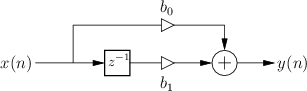
Figure B.1 gives the signal flow graph for the general one-zero filter. The frequency response for the one-zero filter may be found by the following steps:

By factoring out
![]() from the frequency response, to
balance the exponents of
from the frequency response, to
balance the exponents of ![]() , we can get this closer to polar form as
follows:
, we can get this closer to polar form as
follows:
 |
We now apply the general equations given in
Chapter 7 for filter gain ![]() and filter phase
and filter phase
![]() as a function of frequency:
as a function of frequency:
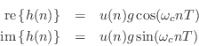
![\begin{eqnarray*}
H(e^{j\omega T}) &=& b_0 + b_1e^{-j\omega T}\\
&=& b_0 + b_1...
...left[\frac{-b_1 \sin(\omega T)}{b_0 + b_1 \cos(\omega T)}\right]
\end{eqnarray*}](http://www.dsprelated.com/josimages_new/filters/img1343.png)
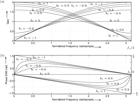
A plot of ![]() and
and
![]() for
for ![]() and various
real values of
and various
real values of ![]() , is given in Fig.B.2. The filter has a zero
at
, is given in Fig.B.2. The filter has a zero
at
![]() in the
in the ![]() plane, which is always on the
real axis. When a point on the unit circle comes close to the zero of
the transfer function the filter gain at that frequency is
low. Notice that one real zero can basically make either a highpass
(
plane, which is always on the
real axis. When a point on the unit circle comes close to the zero of
the transfer function the filter gain at that frequency is
low. Notice that one real zero can basically make either a highpass
(
![]() ) or a lowpass filter (
) or a lowpass filter (
![]() ). For the phase
response calculation using the graphical method, it is necessary to
include the pole at
). For the phase
response calculation using the graphical method, it is necessary to
include the pole at ![]() .
.
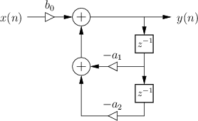
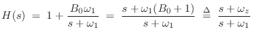
One-Pole
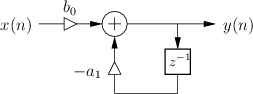
Fig.B.3 gives the signal flow graph for the general one-pole filter. The road to the frequency response goes as follows:
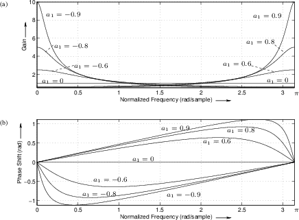 |
The one-pole filter has a transfer function (hence frequency response) which is the reciprocal of that of a one-zero. The analysis is thus quite analogous. The frequency response in polar form is given by
![\begin{eqnarray*}
G(\omega) &=& \frac{\vert b_0\vert}{\sqrt{[1 + a_1 \cos(\omega...
... + a_1 \cos(\omega T)}\right], & b_0<0 \\
\end{array} \right..
\end{eqnarray*}](http://www.dsprelated.com/josimages_new/filters/img1351.png)
A plot of the frequency response in polar form for ![]() and
various values of
and
various values of ![]() is given in Fig.B.4.
is given in Fig.B.4.
The filter has a pole at ![]() , in the
, in the ![]() plane (and a zero at
plane (and a zero at ![]() = 0). Notice that the one-pole exhibits
either a lowpass or a highpass frequency response, like the
one-zero. The lowpass character occurs when the pole is near the point
= 0). Notice that the one-pole exhibits
either a lowpass or a highpass frequency response, like the
one-zero. The lowpass character occurs when the pole is near the point
![]() (dc), which happens when
(dc), which happens when ![]() approaches
approaches ![]() . Conversely,
the highpass nature occurs when
. Conversely,
the highpass nature occurs when ![]() is positive.
is positive.
The one-pole filter section can achieve much more drastic differences
between the gain at high frequencies and the gain at low frequencies
than can the one-zero filter. This difference is achieved in the
one-pole by gain boost in the passband rather than
attenuation in the stopband; thus it is usually desirable when
using a one-pole filter to set ![]() to a small value, such as
to a small value, such as
![]() , so that the peak gain is 1 or so. When the peak gain is 1,
the filter is unlikely to overflow.B.1
, so that the peak gain is 1 or so. When the peak gain is 1,
the filter is unlikely to overflow.B.1
Finally, note that the one-pole filter is stable if and only if
![]() .
.
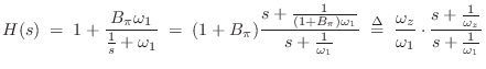
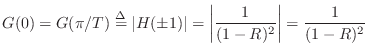
Two-Pole
The signal flow graph for the general two-pole filter is given in Fig.B.5. We proceed as usual with the general analysis steps to obtain the following:
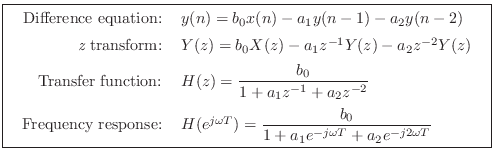
The numerator of ![]() is a constant, so there are no zeros other
than two at the origin of the
is a constant, so there are no zeros other
than two at the origin of the ![]() plane.
plane.
The coefficients ![]() and
and ![]() are called the denominator
coefficients, and they determine the two poles of
are called the denominator
coefficients, and they determine the two poles of ![]() .
Using the quadratic formula, the poles are found to be located at
.
Using the quadratic formula, the poles are found to be located at
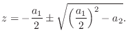
When both poles are real, the two-pole can be analyzed simply as a cascade of two one-pole sections, as in the previous section. That is, one can multiply pointwise two magnitude plots such as Fig.B.4a, and add pointwise two phase plots such as Fig.B.4b.
When the poles are complex, they can be written as
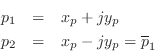
since they must form a complex-conjugate pair when ![]() and
and ![]() are real.
We may express them in polar form
as
are real.
We may express them in polar form
as
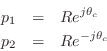
where
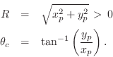
![]() is the pole radius, or distance from the origin in the
is the pole radius, or distance from the origin in the
![]() -plane. As discussed in Chapter 8, we must have
-plane. As discussed in Chapter 8, we must have ![]() for
stability of the two-pole filter. The angles
for
stability of the two-pole filter. The angles
![]() are the
poles' respective angles in the
are the
poles' respective angles in the ![]() plane. The pole angle
plane. The pole angle
![]() corresponds to the pole frequency
corresponds to the pole frequency ![]() via the
relation
via the
relation
If ![]() is sufficiently large (but less than 1 for stability), the
filter exhibits a resonanceB.2 at
radian frequency
is sufficiently large (but less than 1 for stability), the
filter exhibits a resonanceB.2 at
radian frequency
![]() . We may call
. We may call
![]() or
or ![]() the center frequency of the
resonator. Note, however, that the resonance frequency is not usually
the precise frequency of peak-gain in a two-pole resonator (see
Fig.B.9 on page
the center frequency of the
resonator. Note, however, that the resonance frequency is not usually
the precise frequency of peak-gain in a two-pole resonator (see
Fig.B.9 on page ![]() ).
The peak of the amplitude response is usually a little different
because each pole sits on the other's ``skirt,'' which is slanted.
(See §B.1.5 and §B.6 for an elaboration of this point.)
).
The peak of the amplitude response is usually a little different
because each pole sits on the other's ``skirt,'' which is slanted.
(See §B.1.5 and §B.6 for an elaboration of this point.)
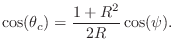
Using polar form for the (complex) poles, the two-pole transfer
function can be expressed as
Comparing this to the transfer function derived from the difference equation, we may identify
The difference equation can thus be rewritten as
Note that coefficient ![]() depends only on the pole radius R (which
determines damping) and is independent of the resonance frequency,
while
depends only on the pole radius R (which
determines damping) and is independent of the resonance frequency,
while ![]() is a function of both. As a result, we may retune
the resonance frequency of the two-pole filter section by modifying
is a function of both. As a result, we may retune
the resonance frequency of the two-pole filter section by modifying
![]() only.
only.
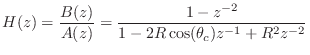
The gain at the resonant frequency
![]() , is found by
substituting
, is found by
substituting
![]() into
Eq.
into
Eq.![]() (B.1) to get
(B.1) to get
See §B.6 for details on how the resonance
gain (and peak gain) can be normalized as the tuning of ![]() is
varied in real time.
is
varied in real time.
Since the radius of both poles is ![]() , we must have
, we must have ![]() for filter
stability (§8.4). The
closer
for filter
stability (§8.4). The
closer ![]() is to 1, the higher the gain at the resonant frequency
is to 1, the higher the gain at the resonant frequency
![]() . If
. If ![]() , the filter degenerates to the form
, the filter degenerates to the form
![]() , which is a nothing but a scale factor. We can say that
when the two poles move to the origin of the
, which is a nothing but a scale factor. We can say that
when the two poles move to the origin of the ![]() plane, they are
canceled by the two zeros there.
plane, they are
canceled by the two zeros there.
Resonator Bandwidth in Terms of Pole Radius
The magnitude ![]() of a complex pole determines the
damping or bandwidth of the resonator. (Damping may be
defined as the reciprocal of the bandwidth.)
of a complex pole determines the
damping or bandwidth of the resonator. (Damping may be
defined as the reciprocal of the bandwidth.)
As derived in §8.5, when ![]() is close to 1, a reasonable
definition of 3dB-bandwidth
is close to 1, a reasonable
definition of 3dB-bandwidth ![]() is provided by
is provided by

where
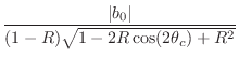
Figure B.6 shows a family of frequency responses for the
two-pole resonator obtained by setting ![]() and varying
and varying ![]() . The
value of
. The
value of ![]() in all cases is
in all cases is ![]() , corresponding to
, corresponding to
![]() . The analytic expressions for amplitude and phase response are
. The analytic expressions for amplitude and phase response are
![\begin{eqnarray*}
G(\omega)\! &=&
\!\frac{b_0}{\sqrt{[1 + a_1 \cos(\omega T) + a...
... + a_1 \cos(\omega T) + a_2 \cos(2\omega T)}\right]\qquad(b_0>0)
\end{eqnarray*}](http://www.dsprelated.com/josimages_new/filters/img1385.png)
where
![]() and
and ![]() .
.
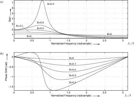 |
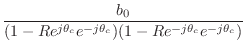
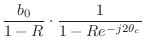
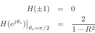
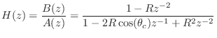
Two-Zero
The signal flow graph for the general two-zero filter is given in Fig.B.7, and the derivation of frequency response is as follows:
![\fbox{
\begin{tabular}{rl}
Difference equation: & $y(n) = b_0 x(n) + b_1 x(n-1) ...
...+ b_1 \cos(\omega T) + b_2 \cos(2\omega T)}\right]$
\end{tabular}\vspace{10pt}
}](http://www.dsprelated.com/josimages_new/filters/img1389.png)
As discussed in §5.1,
the parameters ![]() and
and ![]() are called the numerator
coefficients, and they determine the two zeros. Using the
quadratic formula for finding the roots of a second-order polynomial,
we find that the zeros are located at
are called the numerator
coefficients, and they determine the two zeros. Using the
quadratic formula for finding the roots of a second-order polynomial,
we find that the zeros are located at

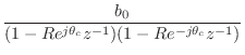
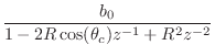
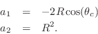
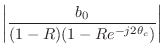
Forming a general two-zero transfer function in factored form gives
![\begin{eqnarray*}
H(z) &=& b_0 (1 - Re^{j\theta_c} z^{-1}) (1 - Re^{-j\theta_c} z^{-1})\\
&=& b_0 [1 - 2R\cos(\theta_c) z^{-1}+ R^2 z^{-2}]
\end{eqnarray*}](http://www.dsprelated.com/josimages_new/filters/img1397.png)
from which we identify
![]() and
and
![]() , so that
, so that
The approximate relation between bandwidth and ![]() given in
Eq.
given in
Eq.![]() (B.5) for the two-pole resonator now applies to the notch
width in the two-zero filter.
(B.5) for the two-pole resonator now applies to the notch
width in the two-zero filter.
Figure B.8 gives some two-zero frequency responses obtained by
setting ![]() to 1 and varying
to 1 and varying ![]() . The value of
. The value of ![]() , is again
, is again
![]() . Note that the response is exactly analogous to the two-pole
resonator with notches replacing the resonant peaks. Since the plots
are on a linear magnitude scale, the two-zero amplitude response
appears as the reciprocal of a two-pole response. On a dB scale, the
two-zero response is an upside-down two-pole response.
. Note that the response is exactly analogous to the two-pole
resonator with notches replacing the resonant peaks. Since the plots
are on a linear magnitude scale, the two-zero amplitude response
appears as the reciprocal of a two-pole response. On a dB scale, the
two-zero response is an upside-down two-pole response.
 |
Complex Resonator
Normally when we need a resonator, we think immediately of the two-pole resonator. However, there is also a complex one-pole resonator having the transfer function
where
Since the impulse response is the inverse z transform of the
transfer function, we can write down the impulse response of the
complex one-pole resonator by recognizing Eq.![]() (B.6) as the
closed-form sum of an infinite geometric series, yielding
(B.6) as the
closed-form sum of an infinite geometric series, yielding
![$\displaystyle u(n) \isdef \left\{\begin{array}{ll}
1, & n\geq 0 \\ [5pt]
0, & n<0 \\
\end{array}\right.
$](http://www.dsprelated.com/josimages_new/filters/img1406.png)
These may be called phase-quadrature sinusoids, since their phases differ by 90 degrees. The phase quadrature relationship for two sinusoids means that they can be regarded as the real and imaginary parts of a complex sinusoid.
By allowing ![]() to be complex,
to be complex,
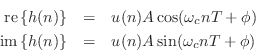
The frequency response of the complex one-pole resonator differs from
that of the two-pole real resonator in that the resonance
occurs only for one positive or negative frequency ![]() , but not
both. As a result, the resonance frequency
, but not
both. As a result, the resonance frequency ![]() is also the
frequency where the peak-gain occurs; this is only true in
general for the complex one-pole resonator. In particular, the peak
gain of a real two-pole filter does not occur exactly at resonance, except
when
is also the
frequency where the peak-gain occurs; this is only true in
general for the complex one-pole resonator. In particular, the peak
gain of a real two-pole filter does not occur exactly at resonance, except
when
![]() ,
, ![]() , or
, or ![]() . See
§B.6 for more on peak-gain versus resonance-gain (and how to
normalize them in practice).
. See
§B.6 for more on peak-gain versus resonance-gain (and how to
normalize them in practice).
Two-Pole Partial Fraction Expansion
Note that every real two-pole resonator can be broken up into a sum of two complex one-pole resonators:
where
![\includegraphics[width=\twidth ]{eps/tppfe}](http://www.dsprelated.com/josimages_new/filters/img1419.png) |
To show Eq.![]() (B.7) is always true, let's solve in general for
(B.7) is always true, let's solve in general for ![]() and
and ![]() given
given ![]() and
and ![]() . Recombining the right-hand side
over a common denominator and equating numerators gives
. Recombining the right-hand side
over a common denominator and equating numerators gives
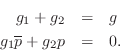
The solution is easily found to be
where we have assumed
im![]() , as necessary to have a
resonator in the first place.
, as necessary to have a
resonator in the first place.
Breaking up the two-pole real resonator into a parallel sum of two complex one-pole resonators is a simple example of a partial fraction expansion (PFE) (discussed more fully in §6.8).
Note that the inverse z transform of a sum of one-pole transfer
functions can be easily written down by inspection. In particular,
the impulse response of the PFE of the two-pole resonator (see
Eq.![]() (B.7)) is clearly
(B.7)) is clearly
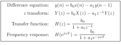
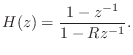
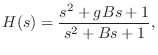
The BiQuad Section
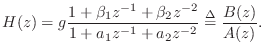
The term ``biquad'' is short for ``bi-quadratic'', and is a common name for a two-pole, two-zero digital filter. The transfer function of the biquad can be defined as
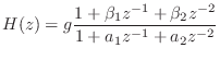
where
As derived in §B.1.3, for real second-order polynomials having
complex roots, it is often convenient to express the polynomial
coefficients in terms of the radius ![]() and angle
and angle ![]() of the
positive-frequency pole. For example, denoting the denominator
polynomial by
of the
positive-frequency pole. For example, denoting the denominator
polynomial by
![]() , we have
, we have
As discussed on page ![]() , a common setting for the zeros when
making a resonator is to place one at
, a common setting for the zeros when
making a resonator is to place one at ![]() (dc) and the other at
(dc) and the other at
![]() (half the sampling rate), i.e.,
(half the sampling rate), i.e., ![]() and
and
![]() in
Eq.
in
Eq.![]() (B.8) above
(B.8) above
![]() .
This zero placement normalizes the peak gain of the resonator if it is
swept using the
.
This zero placement normalizes the peak gain of the resonator if it is
swept using the ![]() parameter.
parameter.
Using the shift theorem for z transforms, the difference equation for the biquad can be written by inspection of the transfer function as
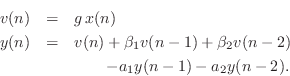
where ![]() denotes the input signal sample at time
denotes the input signal sample at time ![]() , and
, and ![]() is the output signal. This is the form that is typically implemented
in software. It is essentially the direct-form I implementation. (To obtain the official
direct-form I structure, the overall gain
is the output signal. This is the form that is typically implemented
in software. It is essentially the direct-form I implementation. (To obtain the official
direct-form I structure, the overall gain ![]() must be not be pulled
out separately, resulting in feedforward coefficients
must be not be pulled
out separately, resulting in feedforward coefficients
![]() instead. See Chapter 9 for more about
filter implementation forms.)
instead. See Chapter 9 for more about
filter implementation forms.)
Biquad Software Implementations
In matlab, an efficient biquad section is implemented by calling
outputsignal = filter(B,A,inputsignal);
where
![\begin{eqnarray*}
\texttt{B} &=& [g, g\beta_1, g\beta_2],\\
\texttt{A} &=& [1, a_1, a_2].
\end{eqnarray*}](http://www.dsprelated.com/josimages_new/filters/img1436.png)
A complete C++ class implementing a biquad filter section is included in the free, open-source Synthesis Tool Kit (STK) [15]. (See the BiQuad STK class.)
Figure B.10 lists an example biquad implementation in the C programming language.
typedef double *pp; // pointer to array of length NTICK typedef word double; // signal and coefficient data type typedef struct _biquadVars { pp output; pp input; word s2; word s1; word gain; word a2; word a1; word b2; word b1; } biquadVars; void biquad(biquadVars *a) { int i; dbl A; word s0; for (i=0; i<NTICK; i++) { A = a->gain * a->input[i]; A -= a->a1 * a->s1; A -= a->a2 * a->s2; s0 = A; A += a->b1 * a->s1; a->output[i] = a->b2 * a->s2 + A; a->s2 = a->s1; a->s1 = s0; } } |
Allpass Filter Sections
The allpass filter passes all frequencies with equal gain. This
is in contrast with a lowpass filter, which passes only low
frequencies, a highpass which passes high-frequencies, and a bandpass
filter which passes an interval of frequencies. An allpass filter may
have any phase response. The only requirement is that its amplitude
response be constant. Normally, this constant is
![]() .
.
From a physical modeling point of view, a unity-gain allpass filter
models a lossless system in the sense
that it preserves signal energy. Specifically, if ![]() denotes the input to an allpass filter
denotes the input to an allpass filter ![]() , and if
, and if ![]() denotes
its output, then we have
denotes
its output, then we have
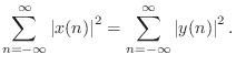
This equation says that the total energy out equals the total energy in. No energy was created or destroyed by the filter. All an allpass filter can do is delay the sinusoidal components of a signal by differing amounts.
Appendix C proves that Eq.![]() (B.9) holds if and only if
(B.9) holds if and only if
The Biquad Allpass Section
The general biquad transfer function was given in Eq.![]() (B.8) to be
(B.8) to be
In terms of the poles and zeros of a filter
![]() , an
allpass filter must have a zero at
, an
allpass filter must have a zero at ![]() for each pole at
for each pole at ![]() .
That is if the denominator
.
That is if the denominator ![]() satisfies
satisfies ![]() , then the
numerator polynomial
, then the
numerator polynomial ![]() must satisfy
must satisfy ![]() . (Show this in
the one-pole case.) Therefore, defining
. (Show this in
the one-pole case.) Therefore, defining
![]() takes care of
this property for all roots of
takes care of
this property for all roots of ![]() (all poles). However, since we
prefer that
(all poles). However, since we
prefer that ![]() be a polynomial in
be a polynomial in ![]() , we define
, we define
![]() , where
, where ![]() is the order of
is the order of ![]() (the number of poles).
(the number of poles).
![]() is then the flip of
is then the flip of ![]() .
.
For further discussion and examples of allpass filters (including muli-input, multi-output allpass filters), see Appendix C. Analog allpass filters are defined and discussed in §E.8.
Allpass Filter Design
There is a fairly large literature thread on the topic of allpass filter design. Generally, they fall into two main categories: parametric and nonparametric methods. Parametric methods can produce allpass filters with optimal group-delay characteristics [42,41]. Nonparametric methods, while suboptimal, can design very large-order allpass filters, and errors can usually be made arbitrarily small by increasing the order [100,70,1], [78, pp. 60,172]. In music applications, it is usually the case that the ``optimality'' criterion is unknown because it depends on aspects of sound perception (see, for example, [35,72]). As a result, perceptually weighted nonparametric methods can often outperform optimal parametric methods in terms of cost/performance. For a nonparametric method that can design very high-order allpass filters according to highly flexible criteria, see [1].
DC Blocker
The dc blocker is an indispensable tool in digital waveguide modeling [86] and other applications.B.4 It is often needed to remove the dc component of the signal circulating in a delay-line loop. It is also often an important tool in multi-track recording, where dc components in the various tracks can add up and overflow the mix.
The dc blocker is a small recursive filter specified by the difference equation
Thus, there is a zero at dc (
DC Blocker Frequency Response
Figure B.11 shows the frequency response of the dc blocker
for several values of ![]() . The same plots are given over a
log-frequency scale in Fig.B.12. The corresponding
pole-zero diagrams are shown in Fig.B.13. As
. The same plots are given over a
log-frequency scale in Fig.B.12. The corresponding
pole-zero diagrams are shown in Fig.B.13. As ![]() approaches
approaches
![]() , the notch at dc gets narrower and narrower. While this may seem
ideal, there is a drawback, as shown in Fig.B.14 for the
case of
, the notch at dc gets narrower and narrower. While this may seem
ideal, there is a drawback, as shown in Fig.B.14 for the
case of ![]() : The impulse response duration increases as
: The impulse response duration increases as ![]() .
While the ``tail'' of the impulse response lengthens as
.
While the ``tail'' of the impulse response lengthens as ![]() approaches
1, its initial magnitude decreases. At the limit,
approaches
1, its initial magnitude decreases. At the limit, ![]() , the pole and
zero cancel at all frequencies, the impulse response becomes an
impulse, and the notch disappears.
, the pole and
zero cancel at all frequencies, the impulse response becomes an
impulse, and the notch disappears.
![\includegraphics[width=\twidth ]{eps/dcblockerfr}](http://www.dsprelated.com/josimages_new/filters/img1459.png) |
![\includegraphics[width=\twidth ]{eps/dcblockerfrlf}](http://www.dsprelated.com/josimages_new/filters/img1460.png) |
![\includegraphics[width=\twidth]{eps/dcblockerpz}](http://www.dsprelated.com/josimages_new/filters/img1461.png) |
![\includegraphics[width=\twidth ]{eps/dcblockerir}](http://www.dsprelated.com/josimages_new/filters/img1462.png)
Note that the amplitude response in Fig.B.11a and
Fig.B.12a exceeds 1 at half the sampling rate.
This maximum gain is given by
![]() . In applications for
which the gain must be bounded by 1 at all frequencies, the dc blocker
may be scaled by the inverse of this maximum gain to yield
. In applications for
which the gain must be bounded by 1 at all frequencies, the dc blocker
may be scaled by the inverse of this maximum gain to yield
![\begin{eqnarray*}
H(z) &=& g\frac{1-z^{-1}}{1-Rz^{-1}}\\
y(n) &=& g[x(n) - x(n-1)] + R\, y(n-1), \quad\hbox{where}\\
g &\isdef & \frac{1+R}{2}.
\end{eqnarray*}](http://www.dsprelated.com/josimages_new/filters/img1464.png)
DC Blocker Software Implementations
In plain C, the difference equation for the dc blocker could be written as follows:
  y = x - xm1 + 0.995 * ym1;
  xm1 = x;
  ym1 = y;
Here, x denotes the current input sample, and y denotes the current output sample. The variables xm1 and ym1 hold once-delayed input and output samples, respectively (and are typically initialized to zero). In this implementation, the pole is fixed at
A complete C++ class implementing a dc blocking filter is included in the free, open-source Synthesis Tool Kit (STK) [15]. (See the DCBlock STK class.)
For a discussion of issues and solutions related to fixed-point implementations, see [7].
Low and High Shelving Filters
The analog transfer function for a low shelf is given by [103]
A high shelf is obtained from a low shelf by the conformal mapping
![]() , which interchanges high and low frequencies, i.e.,
, which interchanges high and low frequencies, i.e.,
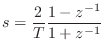
To convert these analog-filter transfer functions to digital form, we apply the bilinear transform:
Low and high shelf filters are typically implemented in series, and are typically used to give a little boost or cut at the extreme low or high end (of the spectrum), respectively. To provide a boost or cut near other frequencies, it is necessary to go to (at least) a second-order section, often called a ``peaking equalizer,'' as described in §B.5 below.
Exercise
Perform the bilinear transform defined above and calculate the
coefficients of a first-order digital low shelving filter. Find the
pole and zero as a function of ![]() ,
, ![]() , and
, and ![]() . Set
. Set ![]() and verify that you get a gain of
and verify that you get a gain of ![]() . Set
. Set ![]() and verify that
you get a gain of 1 there.
and verify that
you get a gain of 1 there.
Peaking Equalizers
A peaking equalizer filter section provides a boost or cut in the vicinity of some center frequency. It may also be called a parametric equalizer section. The gain far away from the boost or cut is unity, so it is convenient to combine a number of such sections in series. Additionally, a high and/or low shelf (§B.4 above) are nice to include in series with one's peaking eq sections.
The analog transfer function for a peak filter is given by [103,5,6]
It is easy to show that both zeros and both poles are on the unit
circle in the left-half ![]() plane, and when
plane, and when ![]() (a ``cut''), the
zeros are closer to the
(a ``cut''), the
zeros are closer to the ![]() axis than the poles.
axis than the poles.
Again, the bilinear transform can be used to convert the analog peaking equalizer section to digital form.
Figure B.15 gives a matlab listing for a peaking EQ section. Figure B.16 shows the resulting plot for an example call:
boost(2,0.25,0.1);The frequency-response utility myfreqz, listed in Fig.7.1, can be substituted for freqz.
function [B,A] = boost(gain,fc,bw,fs); %BOOST - Design a boost filter at given gain, center % frequency fc, bandwidth bw, and sampling rate fs % (default = 1). % % J.O. Smith 11/28/02 % Reference: Zolzer: Digital Audio Signal Processing, p. 124 if nargin<4, fs = 1; end if nargin<3, bw = fs/10; end Q = fs/bw; wcT = 2*pi*fc/fs; K=tan(wcT/2); V=gain; b0 = 1 + V*K/Q + K^2; b1 = 2*(K^2 - 1); b2 = 1 - V*K/Q + K^2; a0 = 1 + K/Q + K^2; a1 = 2*(K^2 - 1); a2 = 1 - K/Q + K^2; A = [a0 a1 a2] / a0; B = [b0 b1 b2] / a0; if nargout==0 figure(1); freqz(B,A); title('Boost Frequency Response') end |
![\includegraphics[width=\twidth]{eps/tboost}](http://www.dsprelated.com/josimages_new/filters/img1489.png) |
A Faust implementation of the peaking equalizer is available as the function peak_eq in filter.lib distributed with Faust (Appendix K) starting with version 0.9.9.4k-par.
Time-Varying Two-Pole Filters
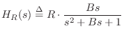
It is quite common to want to vary the resonance frequency of a resonator in real time. This is a special case of a tunable filter. In the pre-digital days of analog synthesizers, filter modules were tuned by means of control voltages, and were thus called voltage-controlled filters (VCF). In the digital domain, control voltages are replaced by time-varying filter coefficients. In the time-varying case, the choice of filter structure has a profound effect on how the filter characteristics vary with respect to coefficient variations. In this section, we will take a look at the time-varying two-pole resonator.
Evaluating the transfer function of the two-pole resonator
(Eq.![]() (B.1)) at the point
(B.1)) at the point
![]() on the unit circle
(the filter's resonance frequency
on the unit circle
(the filter's resonance frequency
![]() ) yields a gain at resonance equal to
) yields a gain at resonance equal to
For simplicity, let
Since
An important fact we can now see is that the gain at resonance depends markedly on the resonance frequency. In particular, the ratio of the two cases just analyzed is

Note that the ratio of the dc resonance gain to the ![]() resonance
gain is unbounded! The sharper the resonance (the closer
resonance
gain is unbounded! The sharper the resonance (the closer ![]() is to 1), the greater the disparity in the gain.
is to 1), the greater the disparity in the gain.
Figure B.17 illustrates a number of resonator frequency responses
for the case ![]() . (Resonators in practice may use values of
. (Resonators in practice may use values of ![]() even closer to 1 than this--even the case
even closer to 1 than this--even the case ![]() is used for making
recursive digital sinusoidal oscillators [90].) For
resonator tunings at dc and
is used for making
recursive digital sinusoidal oscillators [90].) For
resonator tunings at dc and ![]() , we predict the resonance gain to
be
, we predict the resonance gain to
be
![]() dB, and this is what we see in the plot.
When the resonance is tuned to
dB, and this is what we see in the plot.
When the resonance is tuned to ![]() , the gain drops well below 40
dB. Clearly, we will need to compensate this gain variation when
trying to use the two-pole digital resonator as a tunable filter.
, the gain drops well below 40
dB. Clearly, we will need to compensate this gain variation when
trying to use the two-pole digital resonator as a tunable filter.
![\includegraphics[width=\twidth ]{eps/resgain}](http://www.dsprelated.com/josimages_new/filters/img1506.png) |
Figure B.18 shows the same type of plot for the complex
one-pole resonator
![]() , for
, for ![]() and
10 values of
and
10 values of ![]() . In this case, we expect the frequency
response evaluated at the center frequency to be
. In this case, we expect the frequency
response evaluated at the center frequency to be
![]() . Thus, the gain at
resonance for the plotted example is
. Thus, the gain at
resonance for the plotted example is
![]() db for all
tunings. Furthermore, for the complex resonator, the resonance gain
is also exactly equal to the peak gain.
db for all
tunings. Furthermore, for the complex resonator, the resonance gain
is also exactly equal to the peak gain.
![\includegraphics[width=\twidth ]{eps/cresgain}](http://www.dsprelated.com/josimages_new/filters/img1509.png) |
Normalizing Two-Pole Filter Gain at Resonance
The question we now pose is how to best compensate the tunable
two-pole resonator of §B.1.3 so that its peak gain is the same for
all tunings. Looking at Fig.B.17, and remembering the graphical
method for determining the amplitude response,B.6 it is intuitively
clear that we can help matters by adding two zeros to the
filter, one near dc and the other near ![]() . A zero exactly at dc
is provided by the term
. A zero exactly at dc
is provided by the term
![]() in the transfer function numerator.
Similarly, a zero at half the sampling rate is provided by the term
in the transfer function numerator.
Similarly, a zero at half the sampling rate is provided by the term
![]() in the numerator. The series combination of both zeros
gives the numerator
in the numerator. The series combination of both zeros
gives the numerator
![]() . The complete
second-order transfer function then becomes
. The complete
second-order transfer function then becomes
Checking the gain for the case
which is better behaved, but now the response falls to zero at dc and
![]() rather than being heavily boosted, as we found in
Eq.
rather than being heavily boosted, as we found in
Eq.![]() (B.12).
(B.12).
Constant Resonance Gain
It turns out it is possible to normalize exactly the
resonance gain of the second-order resonator tuned by a
single coefficient [89]. This is accomplished by
placing the two zeros at
![]() , where
, where ![]() is the radius of
the complex-conjugate pole pair . The transfer function numerator
becomes
is the radius of
the complex-conjugate pole pair . The transfer function numerator
becomes
![]() , yielding
the total transfer function
, yielding
the total transfer function
Thus, the gain at resonance is ![]() for all resonance tunings
for all resonance tunings ![]() .
.
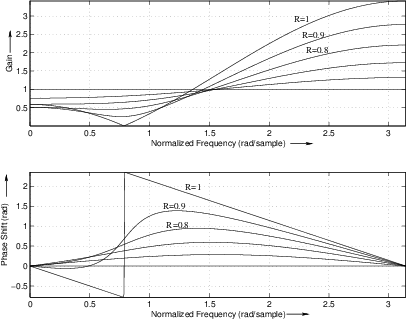
Figure B.19 shows a family of amplitude responses for the
constant resonance-gain two-pole, for various values of ![]() and
and
![]() . We see an excellent improvement in the regularity of the
amplitude response as a function of tuning.
. We see an excellent improvement in the regularity of the
amplitude response as a function of tuning.
![\includegraphics[width=\twidth ]{eps/cgresgain}](http://www.dsprelated.com/josimages_new/filters/img1523.png) |
Peak Gain Versus Resonance Gain
While the constant resonance-gain filter is very well behaved, it is
not ideal, because, while the resonance gain is perfectly
normalized, the peak gain is not. The amplitude-response peak
does not occur exactly at the resonance frequencies
![]() except for the special cases
except for the special cases
![]() ,
, ![]() ,
and
,
and ![]() . At other resonance frequencies, the peak due to one pole
is shifted by the presence of the other pole.
When
. At other resonance frequencies, the peak due to one pole
is shifted by the presence of the other pole.
When ![]() is close to 1, the shifting can be negligible, but in more
damped resonators, e.g., when
is close to 1, the shifting can be negligible, but in more
damped resonators, e.g., when ![]() , there can be a significant
difference between the gain at resonance and the true peak gain.
, there can be a significant
difference between the gain at resonance and the true peak gain.
Figure B.20 shows a family of amplitude responses for the
constant resonance-gain two-pole, for various values of ![]() and
and
![]() . We see that while the gain at resonance is exactly the same
in all cases, the actual peak gain varies somewhat, especially
near dc and
. We see that while the gain at resonance is exactly the same
in all cases, the actual peak gain varies somewhat, especially
near dc and ![]() when the two poles come closest together. A more
pronounced variation in peak gain can be seen in
Fig.B.21, for which the pole radii have been reduced
to
when the two poles come closest together. A more
pronounced variation in peak gain can be seen in
Fig.B.21, for which the pole radii have been reduced
to ![]() .
.
![\includegraphics[width=\twidth ]{eps/cgresgaindamped}](http://www.dsprelated.com/josimages_new/filters/img1526.png) |
![\includegraphics[width=\twidth ]{eps/cgresgaindampedp5}](http://www.dsprelated.com/josimages_new/filters/img1527.png) |
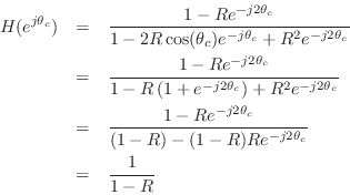
Constant Peak-Gain Resonator
It is surprisingly easy to normalize exactly the peak gain in a second-order resonator tuned by a single coefficient [94]. The filter structure that accomplishes this is the one we already considered in §B.6.1:
That is, the two-pole resonator normalized by zeros at
Real-time audio ``plugins'' based on the constant-peak-gain resonator are developed in Appendix K.
The peak gain is ![]() , so multiplying the transfer function by
, so multiplying the transfer function by
![]() normalizes the peak gain to one for all tunings. It can
also be shown [94] that the peak gain coincides with the
variance gain when the resonator is driven by white noise. That
is, if the variance of the driving noise is
normalizes the peak gain to one for all tunings. It can
also be shown [94] that the peak gain coincides with the
variance gain when the resonator is driven by white noise. That
is, if the variance of the driving noise is ![]() , the variance
of the noise at the resonator output is
, the variance
of the noise at the resonator output is
![]() .
Therefore, scaling the resonator input by
.
Therefore, scaling the resonator input by
![]() will
normalize the resonator such that the output signal power equals the
input signal power when the input signal is white noise.
will
normalize the resonator such that the output signal power equals the
input signal power when the input signal is white noise.
Frequency response overlays for the constant-peak-gain resonator are
shown in Fig.B.23 (![]() ), Fig.B.20
(
), Fig.B.20
(![]() ), and Fig.B.21 (
), and Fig.B.21 (![]() ). While the peak
frequency may be far from the resonance tuning in the more heavily
damped examples, the peak gain is always normalized to unity. The
normalized radian frequency
). While the peak
frequency may be far from the resonance tuning in the more heavily
damped examples, the peak gain is always normalized to unity. The
normalized radian frequency
![]() at which the peak gain
occurs is related to the pole angle
at which the peak gain
occurs is related to the pole angle
![]() by
[94]
by
[94]
When the right-hand side of the above equation exceeds 1 in magnitude, there is no (real) solution for the pole frequency
![\includegraphics[width=\twidth ]{eps/psivsthetac}](http://www.dsprelated.com/josimages_new/filters/img1543.png)
Thus, ![]() must be close to 1 to obtain a resonant peak near dc (a case
commonly needed in audio work) or half the sampling rate (rarely
needed in practice). When
must be close to 1 to obtain a resonant peak near dc (a case
commonly needed in audio work) or half the sampling rate (rarely
needed in practice). When ![]() is much less than 1, the peak frequency
is much less than 1, the peak frequency
![]() cannot leave a small interval near one-fourth the sampling
rate, as can be seen at the far left in Fig.B.22.
cannot leave a small interval near one-fourth the sampling
rate, as can be seen at the far left in Fig.B.22.
Figure B.22 predicts that for ![]() , the lowest peak-gain
frequency should be around
, the lowest peak-gain
frequency should be around
![]() radian per sample.
Figure B.21 agrees with this prediction.
radian per sample.
Figure B.21 agrees with this prediction.
As Figures B.23 through B.25 show, the peak gain remains
constant even at very low and very high frequencies, to the extent
they are reachable for a given ![]() . The zeros at dc and
. The zeros at dc and ![]() preclude the possibility of peaks at exactly those frequencies, but
for
preclude the possibility of peaks at exactly those frequencies, but
for ![]() near 1, we can get very close to having a peak at dc or
near 1, we can get very close to having a peak at dc or
![]() , as shown in Figures B.19 and B.20.
, as shown in Figures B.19 and B.20.
![\includegraphics[width=\twidth ]{eps/cpgresgain}](http://www.dsprelated.com/josimages_new/filters/img1546.png) |
![\includegraphics[width=\twidth ]{eps/cpgresgaindamped}](http://www.dsprelated.com/josimages_new/filters/img1547.png) |
![\includegraphics[width=\twidth ]{eps/cpgresgaindampedp5}](http://www.dsprelated.com/josimages_new/filters/img1548.png) |
Four-Pole Tunable Lowpass/Bandpass Filters
As a practical note, it is worth mentioning that in popular analog synthesizers (both real and virtualB.7), VCFs are typically fourth order rather than second order as we have studied here. Perhaps the best known VCF is the Moog VCF. The four-pole Moog VCF is configured to be a lowpass filter with an optional resonance near the cut-off frequency. When the resonance is strong, it functions more like a resonator than a lowpass filter. Various methods for digitizing the Moog VCF are described in [95]. It turns out to be nontrivial to preserve all desirable properties of the analog filter (such as frequency response, order, and control structure), when translated to digital form by standard means.
Elementary Filter Problems
See http://ccrma.stanford.edu/~jos/filtersp/Elementary_Filter_Problems.html.
Next Section:
Allpass Filters
Previous Section:
Background Fundamentals


