


Filter Design by Minimizing the
L2 Equation-Error Norm
One of the simplest formulations of recursive digital filter design is based on minimizing the equation error. This method allows matching of both spectral phase and magnitude. Equation-error methods can be classified as variations of Prony's method [48]. Equation error minimization is used very often in the field of system identification [46,30,78].
The problem of fitting a digital filter to a given spectrum may be formulated as follows:
Given a continuous complex function
![]() ,
corresponding to a causalI.2 desired
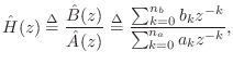
frequency-response, find a stable digital filter of the form
,
corresponding to a causalI.2 desired
frequency-response, find a stable digital filter of the form
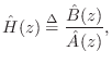
with
![]() given, such that some norm of the error
given, such that some norm of the error
![$\displaystyle \hat{\theta}^T\isdef \left[\hat{b}_0,\hat{b}_1,\ldots\,,\hat{b}_{{n}_b},\hat{a}_1,\hat{a}_2,\ldots\,,\hat{a}_{{n}_a}\right]^T,
$](http://www.dsprelated.com/josimages_new/filters/img2389.png)
The approximate filter ![]() is typically constrained to be stable,
and since positive powers of
is typically constrained to be stable,
and since positive powers of ![]() do not appear in
do not appear in
![]() , stability
implies causality. Consequently, the impulse response of the filter
, stability
implies causality. Consequently, the impulse response of the filter
![]() is zero for
is zero for ![]() . If
. If ![]() were noncausal, all impulse-response components
were noncausal, all impulse-response components
![]() for
for ![]() would be approximated by zero.
would be approximated by zero.
Equation Error Formulation
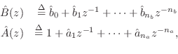
The equation error is defined (in the frequency domain) as
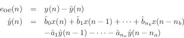
By comparison, the more natural frequency-domain error is the so-called output error:
The names of these errors make the most sense in the time domain. Let
![]() and
and ![]() denote the filter input and output, respectively, at time
denote the filter input and output, respectively, at time
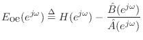
![]() . Then the equation error is the error in the difference equation:
. Then the equation error is the error in the difference equation:
while the output error is the difference between the ideal and approximate filter outputs:
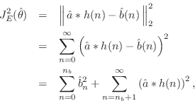
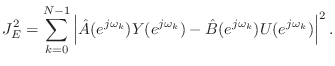
Denote the ![]() norm of the equation error by
norm of the equation error by
where
Note that (I.11) can be expressed as
Error Weighting and Frequency Warping
Audio filter designs typically benefit from an error weighting
function that weights frequencies according
to their audibility. An oversimplified but useful weighting function
is simply ![]() , in which low frequencies are deemed generally
more important than high frequencies. Audio filter designs also
typically improve when using a frequency warping, such as
described in [88,78] (and similar to that
in §I.3.2). In principle, the effect of a frequency-warping can
be achieved using a weighting function, but in practice, the numerical
performance of a frequency warping is often much better.
, in which low frequencies are deemed generally
more important than high frequencies. Audio filter designs also
typically improve when using a frequency warping, such as
described in [88,78] (and similar to that
in §I.3.2). In principle, the effect of a frequency-warping can
be achieved using a weighting function, but in practice, the numerical
performance of a frequency warping is often much better.
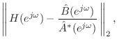
Stability of Equation Error Designs
A problem with equation-error methods is that stability of the filter
design is not guaranteed. When an unstable design is encountered,
one common remedy is to reflect unstable poles inside the unit circle,
leaving the magnitude response unchanged while modifying the phase of the
approximation in an ad hoc manner. This requires polynomial factorization
of
![]() to find the filter poles, which is typically more work
than the filter design itself.
to find the filter poles, which is typically more work
than the filter design itself.
A better way to address the instability problem is to repeat the
filter design employing a bulk delay. This amounts to
replacing
![]() by
by
Unstable equation-error designs are especially likely when
![]() is
noncausal. Since there are no constraints on where the poles of
is
noncausal. Since there are no constraints on where the poles of
![]() can be, one can expect unstable designs for desired
frequency-response functions having a linear phase trend with positive
slope.
can be, one can expect unstable designs for desired
frequency-response functions having a linear phase trend with positive
slope.
In the other direction, experience has shown that best results are obtained
when ![]() is minimum phase, i.e., when all the zeros of
is minimum phase, i.e., when all the zeros of ![]() are
inside the unit circle. For a given magnitude,
are
inside the unit circle. For a given magnitude,
![]() ,
minimum phase gives the maximum concentration of impulse-response energy
near the time origin
,
minimum phase gives the maximum concentration of impulse-response energy
near the time origin ![]() . Consequently, the impulse-response tends to start
large and decay immediately. For non-minimum phase
. Consequently, the impulse-response tends to start
large and decay immediately. For non-minimum phase ![]() , the
impulse-response
, the
impulse-response ![]() may be small for the first
may be small for the first ![]() samples, and the
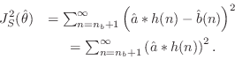
equation error method can yield very poor filters in these cases. To see
why this is so, consider a desired impulse-response
samples, and the
equation error method can yield very poor filters in these cases. To see
why this is so, consider a desired impulse-response ![]() which is zero
for
which is zero
for
![]() , and arbitrary thereafter. Transforming
, and arbitrary thereafter. Transforming ![]() into the
time domain yields
into the
time domain yields
where ``![]() '' denotes convolution, and the additive decomposition
is due the fact that
'' denotes convolution, and the additive decomposition
is due the fact that
![]() for
for
![]() . In this case the
minimum occurs for
. In this case the
minimum occurs for
![]() ! Clearly this is
not a particularly good fit. Thus, the introduction of bulk-delay to guard
against unstable designs is limited by this phenomenon.
! Clearly this is
not a particularly good fit. Thus, the introduction of bulk-delay to guard
against unstable designs is limited by this phenomenon.
It should be emphasized that for minimum-phase
![]() ,
equation-error methods are very effective. It is simple to convert a
desired magnitude response into a minimum-phase frequency-response
by use of cepstral techniques [22,60] (see also the
appendix below), and this is highly recommended when minimizing equation
error. Finally, the error weighting by
,
equation-error methods are very effective. It is simple to convert a
desired magnitude response into a minimum-phase frequency-response
by use of cepstral techniques [22,60] (see also the
appendix below), and this is highly recommended when minimizing equation
error. Finally, the error weighting by
![]() can usually be
removed by a few iterations of the Steiglitz-McBride algorithm.
can usually be
removed by a few iterations of the Steiglitz-McBride algorithm.
An FFT-Based Equation-Error Method
The algorithm below minimizes the equation error in the frequency-domain. As a result, it can make use of the FFT for speed. This algorithm is implemented in Matlab's invfreqz() function when no iteration-count is specified. (The iteration count gives that many iterations of the Steiglitz-McBride algorithm, thus transforming equation error to output error after a few iterations. There is also a time-domain implementation of the Steiglitz-McBride algorithm called stmcb() in the Matlab Signal Processing Toolbox, which takes the desired impulse response as input.)
Given a desired spectrum
![]() at equally spaced frequencies
at equally spaced frequencies
![]() , with
, with ![]() a power of
a power of ![]() ,
it is desired to find a rational digital
filter with
,
it is desired to find a rational digital
filter with ![]() zeros and
zeros and ![]() poles,
poles,
Since ![]() is a quadratic form, the solution is readily obtained by
equating the gradient to zero. An easier derivation follows from minimizing
equation error variance in the time domain and making use of the orthogonality
principle [36].
This may be viewed as a system identification problem where the
known input signal is an impulse, and the known output is the desired
impulse response. A formulation employing an arbitrary known input
is valuable for introducing complex weighting across the frequency grid,
and this general form is presented. A detailed derivation appears in
[78, Chapter 2], and here only the final algorithm is given:
is a quadratic form, the solution is readily obtained by
equating the gradient to zero. An easier derivation follows from minimizing
equation error variance in the time domain and making use of the orthogonality
principle [36].
This may be viewed as a system identification problem where the
known input signal is an impulse, and the known output is the desired
impulse response. A formulation employing an arbitrary known input
is valuable for introducing complex weighting across the frequency grid,
and this general form is presented. A detailed derivation appears in
[78, Chapter 2], and here only the final algorithm is given:
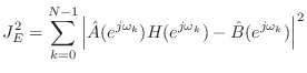
Given spectral output samples
![]() and input
samples
and input
samples
![]() , we minimize
, we minimize
Let
![]() :
:![]() denote the column vector determined
by
denote the column vector determined
by ![]() , for
, for
![]() filled in from top to bottom, and let
filled in from top to bottom, and let
![]() :
:![]() denote the size
denote the size ![]() symmetric Toeplitz matrix consisting of
symmetric Toeplitz matrix consisting of
![]() :
:![]() in its first column.
A nonsymmetric Toeplitz matrix may be specified by its first column and row,
and we use the notation
in its first column.
A nonsymmetric Toeplitz matrix may be specified by its first column and row,
and we use the notation
![]() :
:![]() :
:![]() to denote the
to denote the
![]() by
by ![]() Toeplitz matrix with left-most column
Toeplitz matrix with left-most column
![]() :
:![]() and top row
and top row
![]() :
:![]() .
The inverse Fourier transform of
.
The inverse Fourier transform of
![]() is defined as
is defined as

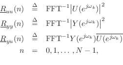
where the overbar denotes complex conjugation, and four corresponding Toeplitz matrices,
![\begin{eqnarray*}
R_{yy} &\isdef & T(\underline{R}_{yy}[0\,\mbox{:}\,{{n}_a}-1])...
...u}^T[-1\,\mbox{:}\,-{{n}_a}])\\
R_{uy} &\isdef & R_{uy}^T , \\
\end{eqnarray*}](http://www.dsprelated.com/josimages_new/filters/img2450.png)
where negative indices are to be interpreted mod ![]() , e.g.,
, e.g.,
![]() .
.
The solution is then
![$\displaystyle \hat{\theta}^\ast = \left[\begin{array}{c} \underline{\hat{B}}^\a...
...,{{n}_b}] \\ [2pt] \underline{R}_{yy}[1\,\mbox{:}\,{{n}_a}] \end{array}\right]
$](http://www.dsprelated.com/josimages_new/filters/img2452.png)
![$\displaystyle \underline{\hat{B}}^\ast \isdef \left[\begin{array}{c} \hat{b}^\a...
...t{a}^\ast _0 \\ [2pt] \vdots \\ [2pt] \hat{a}^\ast _{{n}_a}\end{array}\right],
$](http://www.dsprelated.com/josimages_new/filters/img2453.png)
Prony's Method
There are several variations on equation-error minimization, and some
confusion in terminology exists. We use the definition of Prony's
method given by Markel and Gray [48]. It is equivalent to ``Shank's
method'' [9]. In this method, one first computes the
denominator
![]() by minimizing
by minimizing
This step is equivalent to minimization of ratio error
(as used in linear prediction) for the
all-pole part
![]() , with the first
, with the first ![]() terms of the time-domain
error sum discarded (to get past the influence of the zeros
on the impulse response). When
terms of the time-domain
error sum discarded (to get past the influence of the zeros
on the impulse response). When
![]() , it coincides with the
covariance method of linear prediction [48,47]. This idea for
finding the poles by ``skipping'' the influence of the zeros on the
impulse-response shows up in the stochastic case under the name of modified Yule-Walker equations [11].
, it coincides with the
covariance method of linear prediction [48,47]. This idea for
finding the poles by ``skipping'' the influence of the zeros on the
impulse-response shows up in the stochastic case under the name of modified Yule-Walker equations [11].
Now, Prony's method consists of next minimizing ![]() output error
with the pre-assigned poles given by
output error
with the pre-assigned poles given by
![]() . In other words, the
numerator
. In other words, the
numerator
![]() is found by minimizing
is found by minimizing
The Padé-Prony Method
Another variation of Prony's method, described by Burrus and Parks
[9] consists of using Padé approximation to
find the numerator
![]() after the denominator
after the denominator
![]() has been found
as before. Thus,
has been found
as before. Thus,
![]() is found by matching the first
is found by matching the first ![]() samples of
samples of ![]() , viz.,
, viz.,
![]() . This method is faster, but does not generally give
as good results as the previous version. In particular, the degenerate
example
. This method is faster, but does not generally give
as good results as the previous version. In particular, the degenerate
example
![]() gives
gives
![]() here as did pure
equation error. This method has been applied also in the stochastic
case [11].
here as did pure
equation error. This method has been applied also in the stochastic
case [11].
On the whole, when
![]() is causal and minimum phase (the ideal
situation for just about any stable filter-design method), the
variants on equation-error minimization described in this section
perform very similarly. They are all quite fast, relative to
algorithms which iteratively minimize output error, and the
equation-error method based on the FFT above is generally fastest.
is causal and minimum phase (the ideal
situation for just about any stable filter-design method), the
variants on equation-error minimization described in this section
perform very similarly. They are all quite fast, relative to
algorithms which iteratively minimize output error, and the
equation-error method based on the FFT above is generally fastest.
Next Section:
Time Plots: myplot.m
Previous Section:
Digitizing Analog Filters with the Bilinear Transformation


