


Phase and Group Delay
In the previous sections we looked at the two most important
frequency-domain representations for LTI digital filters, the transfer
function ![]() and the frequency response:
and the frequency response:
In the next two sections we look at two alternative forms of the phase response: phase delay and group delay. After considering some examples and special cases, poles and zeros of the transfer function are discussed in the next chapter.
Phase Delay
The phase response
![]() of an LTI filter gives the radian
phase shift added to the phase of each sinusoidal component of the
input signal. It is often more intuitive to consider instead the
phase delay, defined as
of an LTI filter gives the radian
phase shift added to the phase of each sinusoidal component of the
input signal. It is often more intuitive to consider instead the
phase delay, defined as
From a sinewave-analysis point of view, if the input to a filter with
frequency response
![]() is
is
![\begin{eqnarray*}
y(n) &=& G(\omega) \cos[\omega nT + \Theta(\omega)]\\
&=& G(\omega) \cos\{\omega[nT - P(\omega)]\}
\end{eqnarray*}](http://www.dsprelated.com/josimages_new/filters/img889.png)
and it can be clearly seen in this form that the phase delay expresses the phase response as a time delay in seconds.
Phase Unwrapping
In working with phase delay, it is often necessary to ``unwrap''
the phase response
![]() . Phase unwrapping ensures that
all appropriate multiples of
. Phase unwrapping ensures that
all appropriate multiples of ![]() have been included in
have been included in
![]() . We defined
. We defined
![]() simply as the complex
angle of the frequency response
simply as the complex
angle of the frequency response
![]() , and this is not sufficient
for obtaining a phase response which can be converted to true time
delay. If multiples of
, and this is not sufficient
for obtaining a phase response which can be converted to true time
delay. If multiples of ![]() are discarded, as is done in the
definition of complex angle, the phase delay is modified by multiples
of the sinusoidal period. Since LTI filter analysis is based on
sinusoids without beginning or end, one cannot in principle
distinguish between ``true'' phase delay and a phase delay with
discarded sinusoidal periods when looking at a sinusoidal output at
any given frequency. Nevertheless, it is often useful to define the
filter phase response as a continuous function of frequency
with the property that
are discarded, as is done in the
definition of complex angle, the phase delay is modified by multiples
of the sinusoidal period. Since LTI filter analysis is based on
sinusoids without beginning or end, one cannot in principle
distinguish between ``true'' phase delay and a phase delay with
discarded sinusoidal periods when looking at a sinusoidal output at
any given frequency. Nevertheless, it is often useful to define the
filter phase response as a continuous function of frequency
with the property that
![]() or
or ![]() (for real filters). This
specifies how to unwrap the phase response at all frequencies
where the amplitude response is finite and nonzero. When the
amplitude response goes to zero or infinity at some frequency, we can
try to take a limit from below and above that frequency.
(for real filters). This
specifies how to unwrap the phase response at all frequencies
where the amplitude response is finite and nonzero. When the
amplitude response goes to zero or infinity at some frequency, we can
try to take a limit from below and above that frequency.
Matlab and Octave have a function called unwrap() which
implements a numerical algorithm for phase unwrapping.
Figures 7.6.2 and 7.6.2 show the effect of the
unwrap function on the phase response of the example elliptic
lowpass filter of §7.5.2, modified to contract the zeros from
the unit circle to a circle of radius ![]() in the
in the ![]() plane:
plane:
  [B,A] = ellip(4,1,20,0.5); % design lowpass filter
   B = B .* (0.95).^[1:length(B)]; % contract zeros by 0.95
  [H,w] = freqz(B,A);      % frequency response
  theta = angle(H);        % phase response
  thetauw = unwrap(theta); % unwrapped phase response
In Fig.7.6.2, the phase-response minimum has ``wrapped around'' to the top of the plot. In Fig.7.6.2, the phase response is continuous. We have contracted the zeros away from the unit circle in this example, because the phase response really does switch discontinuously by
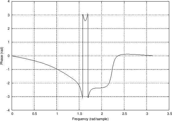
Phase
Response 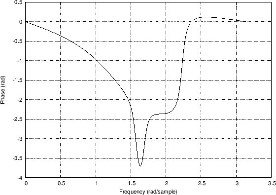
Unwrapped Response
|
Group Delay
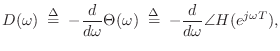
A more commonly encountered representation of filter phase response is called the group delay, defined by
An example of a linear phase response is that of the simplest lowpass
filter,
![]() . Thus, both the phase delay and the group
delay of the simplest lowpass filter are equal to half a sample at
every frequency.
. Thus, both the phase delay and the group
delay of the simplest lowpass filter are equal to half a sample at
every frequency.
For any reasonably smooth phase function, the group delay ![]() may be interpreted as the time delay of the amplitude envelope
of a sinusoid at frequency
may be interpreted as the time delay of the amplitude envelope
of a sinusoid at frequency ![]() [63]. The bandwidth of
the amplitude envelope in this interpretation must be restricted to a
frequency interval over which the phase response is approximately
linear. We derive this result in the next subsection.
[63]. The bandwidth of
the amplitude envelope in this interpretation must be restricted to a
frequency interval over which the phase response is approximately
linear. We derive this result in the next subsection.
Thus, the name ``group delay'' for ![]() refers to the fact that
it specifies the delay experienced by a narrow-band ``group'' of
sinusoidal components which have frequencies within a narrow frequency
interval about
refers to the fact that
it specifies the delay experienced by a narrow-band ``group'' of
sinusoidal components which have frequencies within a narrow frequency
interval about ![]() . The width of this interval is limited to
that over which
. The width of this interval is limited to
that over which ![]() is approximately constant.
is approximately constant.
Derivation of Group Delay as Modulation Delay
Suppose we write a narrowband signal centered at frequency ![]() as
as
where
Using the above frequency-domain expansion of ![]() ,
, ![]() can be
written as
can be
written as
![$\displaystyle x(n) \eqsp a_m(n) e^{j\omega_c n} \eqsp
\left[\frac{1}{2\pi} \int_{-\epsilon}^{\epsilon} A_m(\omega)e^{j\omega n} d\omega\right] e^{j\omega_c n},
$](http://www.dsprelated.com/josimages_new/filters/img908.png)
Assuming the phase response
![\begin{eqnarray*}
y_\omega(n)
&=& \left[G(\omega_c+\omega)A_m(\omega)\right]
e^...
...\right]
e^{j\omega[n-D(\omega_c)]} e^{j\omega_c[n-P(\omega_c)]},
\end{eqnarray*}](http://www.dsprelated.com/josimages_new/filters/img916.png)
where we also used the definition of phase delay,
![]() , in the last step. In this expression we
can already see that the carrier sinusoid is delayed by the phase
delay, while the amplitude-envelope frequency-component is delayed by
the group delay. Integrating over
, in the last step. In this expression we
can already see that the carrier sinusoid is delayed by the phase
delay, while the amplitude-envelope frequency-component is delayed by
the group delay. Integrating over ![]() to recombine the
sinusoidal components (i.e., using a Fourier superposition integral for
to recombine the
sinusoidal components (i.e., using a Fourier superposition integral for
![]() ) gives
) gives
![\begin{eqnarray*}
y(n) &=& \frac{1}{2\pi}\int_{\omega} y_\omega(n) d\omega \\
&...
...)]}\\
&=& a^f[n-D(\omega_c)] \cdot e^{j\omega_c[n-P(\omega_c)]}
\end{eqnarray*}](http://www.dsprelated.com/josimages_new/filters/img918.png)
where ![]() denotes a zero-phase filtering of the amplitude
envelope
denotes a zero-phase filtering of the amplitude
envelope ![]() by
by
![]() . We see that the amplitude
modulation is delayed by
. We see that the amplitude
modulation is delayed by
![]() while the carrier wave is
delayed by
while the carrier wave is
delayed by
![]() .
.
We have shown that, for narrowband signals expressed as in
Eq.![]() (7.6) as a modulation envelope times a sinusoidal carrier, the
carrier wave is delayed by the filter phase delay, while the
modulation is delayed by the filter group delay, provided that the
filter phase response is approximately linear over the narrowband
frequency interval.
(7.6) as a modulation envelope times a sinusoidal carrier, the
carrier wave is delayed by the filter phase delay, while the
modulation is delayed by the filter group delay, provided that the
filter phase response is approximately linear over the narrowband
frequency interval.
Group Delay Examples in Matlab
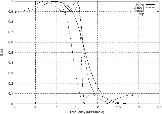
Figure 7.6 compares the group delay responses for a number of classic lowpass filters, including the example of Fig.7.2. The matlab code is listed in Fig.7.5. See, e.g., Parks and Burrus [64] for a discussion of Butterworth, Chebyshev, and Elliptic Function digital filter design. See also §I.2 for details on the Butterworth case. The various types may be summarized as follows:
- Butterworth filters are maximally flat in middle of the passband.
- Chebyshev Type I filters are ``equiripple'' in the passband and ``Butterworth'' in the stopband.
- Chebyshev Type II filters are ``Butterworth'' in the passband and equiripple in the stopband.
- Elliptic function filters are equiripple in both the passband and stopband.
As Fig.7.6.4 indicates, and as is well known, the Butterworth filter has the flattest group delay curve (and most gentle transition from passband to stopband) for the four types compared. The elliptic function filter has the largest amount of ``delay distortion'' near the cut-off frequency (passband edge frequency). Fundamentally, the more abrupt the transition from passband to stopband, the greater the delay-distortion across that transition, for any minimum-phase filter. (Minimum-phase filters are introduced in Chapter 11.) The delay-distortion can be compensated by delay equalization, i.e., adding delay at other frequencies in order approach an overall constant group delay versus frequency. Delay equalization is typically carried out using an allpass filter (defined in §B.2) in series with the filter to be delay-equalized [1].
[Bb,Ab] = butter(4,0.5); % order 4, cutoff at 0.5 * pi Hb=freqz(Bb,Ab); Db=grpdelay(Bb,Ab); [Bc1,Ac1] = cheby1(4,1,0.5); % 1 dB passband ripple Hc1=freqz(Bc1,Ac1); Dc1=grpdelay(Bc1,Ac1); [Bc2,Ac2] = cheby2(4,20,0.5); % 20 dB stopband attenuation Hc2=freqz(Bc2,Ac2); Dc2=grpdelay(Bc2,Ac2); [Be,Ae] = ellip(4,1,20,0.5); % like cheby1 + cheby2 He=freqz(Be,Ae); [De,w]=grpdelay(Be,Ae); figure(1); plot(w,abs([Hb,Hc1,Hc2,He])); grid('on'); xlabel('Frequency (rad/sample)'); ylabel('Gain'); legend('butter','cheby1','cheby2','ellip'); saveplot('../eps/grpdelaydemo1.eps'); figure(2); plot(w,[Db,Dc1,Dc2,De]); grid('on'); xlabel('Frequency (rad/sample)'); ylabel('Delay (samples)'); legend('butter','cheby1','cheby2','ellip'); saveplot('../eps/grpdelaydemo2.eps'); |
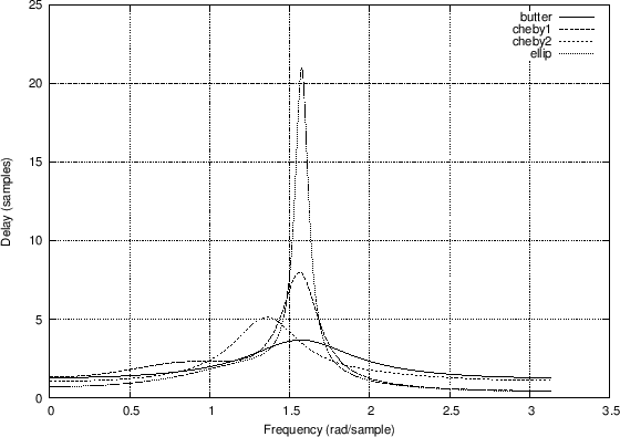
Group Delays
|
Vocoder Analysis
The definitions of phase delay and group delay apply quite naturally to the analysis of the vocoder (``voice coder'') [21,26,54,76]. The vocoder provides a bank of bandpass filters which decompose the input signal into narrow spectral ``slices.'' This is the analysis step. For synthesis (often called additive synthesis), a bank of sinusoidal oscillators is provided, having amplitude and frequency control inputs. The oscillator frequencies are tuned to the filter center frequencies, and the amplitude controls are driven by the amplitude envelopes measured in the filter-bank analysis. (Typically, some data reduction or envelope modification has taken place in the amplitude envelope set.) With these oscillators, the band slices are independently regenerated and summed together to resynthesize the signal.
Suppose we excite only channel ![]() of the vocoder with the input signal
of the vocoder with the input signal
If the phase of each channel filter is linear in frequency within the
passband (or at least across the width of the spectrum
![]() of
of
![]() ), and if each channel filter has a flat amplitude response in
its passband, then the filter output will be, by the analysis of the
previous section,
), and if each channel filter has a flat amplitude response in
its passband, then the filter output will be, by the analysis of the
previous section,
where
Note that a nonlinear phase response generally results in
![]() , and
, and
![]() for
for
![]() . As a result, the dispersive nature of additive synthesis
reconstruction in this case can be seen in Eq.
. As a result, the dispersive nature of additive synthesis
reconstruction in this case can be seen in Eq.![]() (7.8).
(7.8).
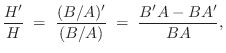
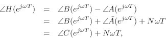
Numerical Computation of Group Delay
The definition of group delay,
A more useful form of the group delay arises from the
logarithmic derivative of the frequency response. Expressing
the frequency response
![]() in polar form as
in polar form as
Since differentiation is linear, the logarithmic derivative becomes
 im
im im
im
In this case, the derivative is simply
![\begin{eqnarray*}
B^\prime(e^{j\omega T}) &\isdef & \frac{d}{d\omega}\left[b_0
...
...b_M e^{-jM\omega T}\right]\\
&\isdef & -jT\,B_r(e^{j\omega T}),
\end{eqnarray*}](http://www.dsprelated.com/josimages_new/filters/img947.png)
where ![]() denotes ``
denotes ``![]() ramped'', i.e., the
ramped'', i.e., the ![]() th coefficient of
the polynomial
th coefficient of
the polynomial ![]() is
is ![]() , for
, for
![]() . In
matlab, we may compute Br from B via the
following statement:
. In
matlab, we may compute Br from B via the
following statement:
Br = B .* [0:M]; % Compute ramped B polynomialThe group delay of an FIR filter
 im
im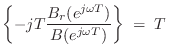 re
re
D = real(fft(Br) ./ fft(B))where the fft, of course, approximates the Discrete Time Fourier Transform (DTFT). Such sampling of the frequency axis by this approximation is information-preserving whenever the number of samples (FFT length) exceeds the polynomial order
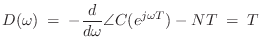
Finally, when there are both poles and zeros, we have
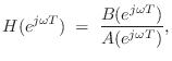
Straightforward differentiation yields
and this can be implemented analogous to the FIR case discussed above. However, a faster algorithm (usually) results from converting the IIR case to the FIR case:
where
C = conv(B,fliplr(conj(A)));It is straightforward to show (Problem 11) that
and the group delay computation thus reduces to the FIR case:
 re
re
Next Section:
Frequency Response Analysis Problems
Previous Section:
Frequency Response as a Ratio of DTFTs


