


Prony's Method
There are several variations on equation-error minimization, and some
confusion in terminology exists. We use the definition of Prony's
method given by Markel and Gray [48]. It is equivalent to ``Shank's
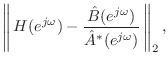
method'' [9]. In this method, one first computes the
denominator
![]() by minimizing
by minimizing
This step is equivalent to minimization of ratio error
(as used in linear prediction) for the
all-pole part
![]() , with the first
, with the first ![]() terms of the time-domain
error sum discarded (to get past the influence of the zeros
on the impulse response). When
terms of the time-domain
error sum discarded (to get past the influence of the zeros
on the impulse response). When
![]() , it coincides with the
covariance method of linear prediction [48,47]. This idea for
finding the poles by ``skipping'' the influence of the zeros on the
impulse-response shows up in the stochastic case under the name of modified Yule-Walker equations [11].
, it coincides with the
covariance method of linear prediction [48,47]. This idea for
finding the poles by ``skipping'' the influence of the zeros on the
impulse-response shows up in the stochastic case under the name of modified Yule-Walker equations [11].
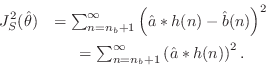
Now, Prony's method consists of next minimizing ![]() output error
with the pre-assigned poles given by
output error
with the pre-assigned poles given by
![]() . In other words, the
numerator
. In other words, the
numerator
![]() is found by minimizing
is found by minimizing
Next Section:
The Padé-Prony Method
Previous Section:
An FFT-Based Equation-Error Method


