


RC Filter Analysis
Referring again to Fig.E.1, let's perform an impedance analysis of the simple RC lowpass filter.
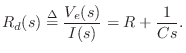
Driving Point Impedance
Taking the Laplace transform of both sides of Eq.![]() (E.1) gives
(E.1) gives
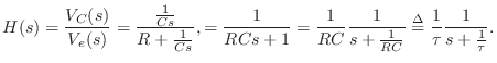
Transfer Function
Since the input and output signals are defined as ![]() and
and
![]() , respectively, the transfer function of this analog
filter is given by, using voltage divider rule,
, respectively, the transfer function of this analog
filter is given by, using voltage divider rule,
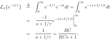
Impulse Response
In the same way that the impulse response of a digital filter is given by the inverse z transform of its transfer function, the impulse response of an analog filter is given by the inverse Laplace transform of its transfer function, viz.,
![$\displaystyle u(t) \isdef \left\{\begin{array}{ll}
1, & t\geq 0 \\ [5pt]
0, & t<0. \\
\end{array}\right.
$](http://www.dsprelated.com/josimages_new/filters/img1814.png)
In more complicated situations, any rational ![]() (ratio of
polynomials in
(ratio of
polynomials in ![]() ) may be expanded into first-order terms by means of
a partial fraction expansion (see §6.8) and each term in
the expansion inverted by inspection as above.
) may be expanded into first-order terms by means of
a partial fraction expansion (see §6.8) and each term in
the expansion inverted by inspection as above.
The Continuous-Time Impulse
The continuous-time impulse response was derived above as the inverse-Laplace transform of the transfer function. In this section, we look at how the impulse itself must be defined in the continuous-time case.
An impulse in continuous time may be loosely defined as any ``generalized function'' having ``zero width'' and unit area under it. A simple valid definition is
![$\displaystyle \delta(t) \isdef \lim_{\Delta \to 0} \left\{\begin{array}{ll} \fr...
...eq t\leq \Delta \\ [5pt] 0, & \hbox{otherwise}. \\ \end{array} \right. \protect$](http://www.dsprelated.com/josimages_new/filters/img1818.png)
More generally, an impulse can be defined as the limit of any pulse shape which maintains unit area and approaches zero width at time 0. As a result, the impulse under every definition has the so-called sifting property under integration,
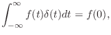
provided
Poles and Zeros
In the simple RC-filter example of §E.4.3, the transfer function is
Next Section:
RLC Filter Analysis
Previous Section:
Inductors


