


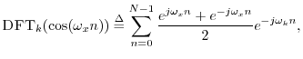
FFT of a Simple Sinusoid
Our first example is an FFT of the simple sinusoid
% Example 1: FFT of a DFT-sinusoid

% Parameters:
N = 64;              % Must be a power of two
T = 1;               % Set sampling rate to 1
A = 1;               % Sinusoidal amplitude
phi = 0;             % Sinusoidal phase
f = 0.25;            % Frequency (cycles/sample)
n = [0:N-1];         % Discrete time axis
x = A*cos(2*pi*n*f*T+phi); % Sampled sinusoid
X = fft(x);          % Spectrum

% Plot time data:
figure(1);
subplot(3,1,1);
plot(n,x,'*k');
ni = [0:.1:N-1];     % Interpolated time axis
hold on;
plot(ni,A*cos(2*pi*ni*f*T+phi),'-k'); grid off;
title('Sinusoid at 1/4 the Sampling Rate');
xlabel('Time (samples)');
ylabel('Amplitude');
text(-8,1,'a)');
hold off;

% Plot spectral magnitude:
magX = abs(X);
fn = [0:1/N:1-1/N];  % Normalized frequency axis
subplot(3,1,2);
stem(fn,magX,'ok'); grid on;
xlabel('Normalized Frequency (cycles per sample))');
ylabel('Magnitude (Linear)');
text(-.11,40,'b)');

% Same thing on a dB scale:
spec = 20*log10(magX); % Spectral magnitude in dB
subplot(3,1,3);
plot(fn,spec,'--ok'); grid on;
axis([0 1 -350 50]);
xlabel('Normalized Frequency (cycles per sample))');
ylabel('Magnitude (dB)');
text(-.11,50,'c)');
cmd = ['print -deps ', '../eps/example1.eps'];
disp(cmd); eval(cmd);
![\includegraphics[width=\twidth]{eps/example1}](http://www.dsprelated.com/josimages_new/mdft/img1494.png) |
The results are shown in Fig.8.1. The time-domain signal is
shown in the upper plot (Fig.8.1a), both in pseudo-continuous
and sampled form. In the middle plot (Fig.8.1b), we see two
peaks in the magnitude spectrum, each at magnitude ![]() on a linear
scale, located at normalized frequencies
on a linear
scale, located at normalized frequencies ![]() and
and
![]() . A spectral peak amplitude of
. A spectral peak amplitude of
![]() is what we
expect, since
is what we
expect, since
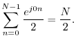
The spectrum should be exactly zero at the other bin numbers. How
accurately this happens can be seen by looking on a dB scale, as shown in
Fig.8.1c. We see that the spectral magnitude in the other bins is
on the order of ![]() dB lower, which is close enough to zero for audio
work
dB lower, which is close enough to zero for audio
work
![]() .
.
Next Section:
FFT of a Not-So-Simple Sinusoid
Previous Section:
Why a DFT is usually called an FFT in practice


