


Geometric Signal Theory
This chapter provides an introduction to the elements of geometric signal theory, including vector spaces, norms, inner products, orthogonality, projection of one signal onto another, and elementary vector space operations. First, however, we will ``get our bearings'' with respect to the DFT.
The DFT
For a length ![]() complex sequence
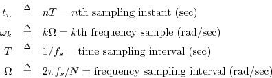
complex sequence ![]() ,
,
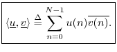
![]() , the
discrete Fourier transform (DFT) is defined by
, the
discrete Fourier transform (DFT) is defined by
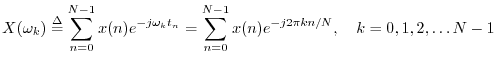
We are now in a position to have a full understanding of the transform kernel:
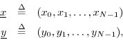
Signals as Vectors
For the DFT, all signals and spectra are length ![]() . A length
. A length ![]() sequence
sequence
![]() can be denoted by
can be denoted by ![]() ,
,
![]() , where
, where ![]() may be
real (
may be
real (
![]() ) or complex (
) or complex (
![]() ). We now wish to regard
). We now wish to regard ![]() as a
vector5.1
as a
vector5.1
![]() in an
in an ![]() dimensional vector space. That is,
each sample
dimensional vector space. That is,
each sample ![]() is regarded as a coordinate in that space.
A vector
is regarded as a coordinate in that space.
A vector
![]() is mathematically a single point in
is mathematically a single point in
![]() -space represented by a list of coordinates
-space represented by a list of coordinates
![]() called an
called an ![]() -tuple. (The
notation
-tuple. (The
notation ![]() means the same thing as
means the same thing as ![]() .) It can be interpreted
geometrically as an arrow in
.) It can be interpreted
geometrically as an arrow in ![]() -space from the origin
-space from the origin
![]() to the point
to the point
![]() .
.
We define the following as equivalent:
The reader comfortable with vectors, vector addition, and vector subtraction may skip to §5.6.
An Example Vector View: 
Consider the example two-sample signal
![]() graphed in
Fig.5.1.
graphed in
Fig.5.1.
![\includegraphics[scale=0.7]{eps/vec2d}](http://www.dsprelated.com/josimages_new/mdft/img689.png)
Under the geometric interpretation of a length ![]() signal, each sample is a
coordinate in the
signal, each sample is a
coordinate in the ![]() dimensional space. Signals which are only two
samples long are not terribly interesting to hear,5.2 but they are easy to
plot geometrically.
dimensional space. Signals which are only two
samples long are not terribly interesting to hear,5.2 but they are easy to
plot geometrically.
Vector Addition
Given two vectors in ![]() , say
, say
the vector sum is defined by
elementwise addition. If we denote the sum by
![]() ,
then we have
,
then we have
![]() for
for
![]() . We could also
write
. We could also
write
![]() for
for
![]() if preferred.
if preferred.
The vector diagram for the sum of two vectors can be found using the
parallelogram rule, as shown in Fig.5.2 for ![]() ,
,
![]() , and
, and
![]() .
.
![\includegraphics[scale=0.7]{eps/vecsum}](http://www.dsprelated.com/josimages_new/mdft/img696.png)
Also shown are the lighter construction lines which complete the
parallelogram started by
![]() and
and
![]() , indicating where the endpoint of the
sum
, indicating where the endpoint of the
sum
![]() lies. Since it is a parallelogram, the two construction lines
are congruent to the vectors
lies. Since it is a parallelogram, the two construction lines
are congruent to the vectors
![]() and
and
![]() . As a result, the vector sum is
often expressed as a triangle by translating the origin of one member
of the sum to the tip of the other, as shown in Fig.5.3.
. As a result, the vector sum is
often expressed as a triangle by translating the origin of one member
of the sum to the tip of the other, as shown in Fig.5.3.
![\includegraphics[scale=0.7]{eps/vecsumr}](http://www.dsprelated.com/josimages_new/mdft/img699.png)
In the figure,
![]() was translated to the tip of
was translated to the tip of
![]() .
This depicts
.
This depicts ![]() , since ``
, since ``![]() picks up where
picks up where ![]() leaves off.''
It is equally valid
to translate
leaves off.''
It is equally valid
to translate
![]() to the tip of
to the tip of
![]() , because vector addition is commutative, i.e.,
, because vector addition is commutative, i.e.,
![]() =
=
![]() .
.
Vector Subtraction
Figure 5.4 illustrates the vector difference
![]() between
between
![]() and
and
![]() . From the coordinates, we compute
. From the coordinates, we compute
![]() .
.
![\includegraphics[scale=0.7]{eps/vecsub}](http://www.dsprelated.com/josimages_new/mdft/img704.png)
Note that the difference vector
![]() may be drawn from the tip of
may be drawn from the tip of
![]() to the
tip of
to the
tip of
![]() rather than from the origin to the point
rather than from the origin to the point ![]() ; this is a
customary practice which emphasizes relationships among vectors, but the
translation in the plot has no effect on the mathematical definition or
properties of the vector. Subtraction, however, is not commutative.
; this is a
customary practice which emphasizes relationships among vectors, but the
translation in the plot has no effect on the mathematical definition or
properties of the vector. Subtraction, however, is not commutative.
To ascertain the proper orientation of the difference vector
![]() ,
rewrite its definition as
,
rewrite its definition as
![]() , and then it is clear that the vector
, and then it is clear that the vector
![]() should be the sum of vectors
should be the sum of vectors
![]() and
and
![]() , hence the arrowhead is on the
correct endpoint. Or remember ``
, hence the arrowhead is on the
correct endpoint. Or remember ``![]() points to
points to ![]() ,'' or ``
,'' or ``![]() is
is ![]() from
from
![]() .''
.''
Scalar Multiplication
A scalar is any constant value used as a scale factor
applied to a vector. Mathematically, all of our scalars will be
either real or complex numbers.5.3 For example, if
![]() denotes a vector of
denotes a vector of ![]() complex elements, and
complex elements, and
![]() denotes a complex scalar,
then
denotes a complex scalar,
then
In signal processing, we think of scalar multiplication as applying some constant scale factor to a signal, i.e., multiplying each sample of the signal by the same constant number. For example, a 6 dB boost can be carried out by multiplying each sample of a signal by 2, in which case 2 is the scalar. When the scalar magnitude is greater than one, it is often called a gain factor, and when it is less than one, an attenuation.
Linear Combination of Vectors
A linear combination of vectors is a sum of scalar
multiples of those vectors. That is, given a set of ![]() vectors
vectors
![]() of the same type,5.4 such as
of the same type,5.4 such as ![]() (they must have the
same number of elements so they can be added), a linear combination is
formed by multiplying each vector by a scalar
(they must have the
same number of elements so they can be added), a linear combination is
formed by multiplying each vector by a scalar ![]() and summing
to produce a new vector
and summing
to produce a new vector
![]() of the same type:
of the same type:
In signal processing, we think of a linear combination as a signal mix. Thus, the output of a mixing console may be regarded as a linear combination of the input signal tracks.
Linear Vector Space
A set of vectors may be called a linear vector space if it is
closed under linear combinations. That is, given any two vectors
![]() and
and
![]() from the set, the linear combination
from the set, the linear combination
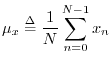
Signal Metrics
This section defines some useful functions of signals (vectors).
The mean of a
signal ![]() (more precisely the ``sample mean'') is defined as the
average value of its samples:5.5
(more precisely the ``sample mean'') is defined as the
average value of its samples:5.5
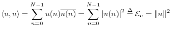
The total energy
of a signal ![]() is defined as the sum of squared moduli:
is defined as the sum of squared moduli:
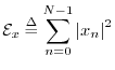
In physics, energy (the ``ability to do work'') and work are in units
of ``force times distance,'' ``mass times velocity squared,'' or other
equivalent combinations of units.5.6 In digital signal processing, physical units are routinely
discarded, and signals are renormalized whenever convenient.
Therefore,
![]() is defined above without regard for constant
scale factors such as ``wave impedance'' or the sampling interval
is defined above without regard for constant
scale factors such as ``wave impedance'' or the sampling interval ![]() .
.
The average power of a signal ![]() is defined as the energy
per sample:
is defined as the energy
per sample:
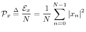
Power is always in physical units of energy per unit time. It therefore makes sense to define the average signal power as the total signal energy divided by its length. We normally work with signals which are functions of time. However, if the signal happens instead to be a function of distance (e.g., samples of displacement along a vibrating string), then the ``power'' as defined here still has the interpretation of a spatial energy density. Power, in contrast, is a temporal energy density.
The root mean square (RMS) level of a signal ![]() is simply
is simply
![]() . However, note that in practice (especially in audio
work) an RMS level is typically computed after subtracting out any
nonzero mean value.
. However, note that in practice (especially in audio
work) an RMS level is typically computed after subtracting out any
nonzero mean value.
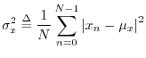
The variance (more precisely the sample variance) of the
signal ![]() is defined as the power of the signal with its mean
removed:5.7
is defined as the power of the signal with its mean
removed:5.7
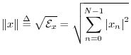
The norm (more specifically, the ![]() norm, or
Euclidean norm) of a signal
norm, or
Euclidean norm) of a signal ![]() is defined as the square root
of its total energy:
is defined as the square root
of its total energy:
Other Lp Norms
Since our main norm is the square root of a sum of squares,
We could equally well have chosen a normalized ![]() norm:
norm:
More generally, the (unnormalized) ![]() norm of
norm of
![]() is defined as
is defined as
 : The
: The  , ``absolute value,'' or ``city block'' norm.
 : The
: The  , ``Euclidean,'' ``root energy,'' or ``least squares'' norm.
 : The
: The
 , ``Chebyshev,'' ``supremum,'' ``minimax,''
or ``uniform'' norm.
, ``Chebyshev,'' ``supremum,'' ``minimax,''
or ``uniform'' norm.
Norm Properties
There are many other possible choices of norm. To qualify as a norm
on ![]() , a real-valued signal-function
, a real-valued signal-function
![]() must
satisfy the following three properties:
must
satisfy the following three properties:
-
 , with

-
-
 ,
,

Banach Spaces
Mathematically, what we are working with so far is called a
Banach space, which is a normed linear vector space. To
summarize, we defined our vectors as any list of ![]() real or complex
numbers which we interpret as coordinates in the
real or complex
numbers which we interpret as coordinates in the ![]() -dimensional
vector space. We also defined vector addition (§5.3) and
scalar multiplication (§5.5) in the obvious way. To have
a linear vector space (§5.7), it must be closed
under vector addition and scalar multiplication (linear
combinations). I.e., given any two vectors
-dimensional
vector space. We also defined vector addition (§5.3) and
scalar multiplication (§5.5) in the obvious way. To have
a linear vector space (§5.7), it must be closed
under vector addition and scalar multiplication (linear
combinations). I.e., given any two vectors
![]() and
and
![]() from the vector space, and given any two scalars
from the vector space, and given any two scalars
![]() and
and
![]() from the field of scalars
from the field of scalars ![]() , the linear
combination
, the linear
combination
![]() must also be in the space. Since
we have used the field of complex numbers
must also be in the space. Since
we have used the field of complex numbers ![]() (or real numbers
(or real numbers
![]() ) to define both our scalars and our vector components, we
have the necessary closure properties so that any linear combination
of vectors from
) to define both our scalars and our vector components, we
have the necessary closure properties so that any linear combination
of vectors from ![]() lies in
lies in ![]() . Finally, the definition of a
norm (any norm) elevates a vector space to a Banach space.
. Finally, the definition of a
norm (any norm) elevates a vector space to a Banach space.
The Inner Product
The inner product (or ``dot product'', or ``scalar product'')
is an operation on two vectors which produces a scalar. Defining an
inner product for a Banach space specializes it to a Hilbert
space (or ``inner product space''). There are many examples of
Hilbert spaces, but we will only need
![]() for this
book (complex length
for this
book (complex length ![]() vectors, and complex scalars).
vectors, and complex scalars).
The inner product between (complex) ![]() -vectors
-vectors
![]() and
and
![]() is
defined by5.9
is
defined by5.9
The complex conjugation of the second vector is done in order that a norm will be induced by the inner product:5.10
Note that the inner product takes
![]() to
to ![]() . That
is, two length
. That
is, two length ![]() complex vectors are mapped to a complex scalar.
complex vectors are mapped to a complex scalar.
Linearity of the Inner Product
Any function
![]() of a vector
of a vector
![]() (which we may call an
operator on
(which we may call an
operator on ![]() ) is said to be linear if for all
) is said to be linear if for all
![]() and
and
![]() , and for all scalars
, and for all scalars ![]() and
and ![]() in
in
![]() ,
,
- additivity:
- homogeneity:
The inner product
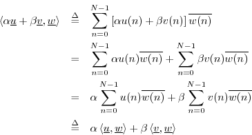
![]() is linear in its first argument, i.e.,
for all
is linear in its first argument, i.e.,
for all
![]() , and for all
, and for all
![]() ,
,
The inner product is also additive in its second argument, i.e.,
The inner product is strictly linear in its second argument with
respect to real scalars ![]() and
and ![]() :
:
Since the inner product is linear in both of its arguments for real scalars, it may be called a bilinear operator in that context.
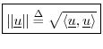
Norm Induced by the Inner Product
We may define a norm on
![]() using the inner product:
using the inner product:
Cauchy-Schwarz Inequality
The Cauchy-Schwarz Inequality (or ``Schwarz Inequality'')
states that for all
![]() and
and
![]() , we have
, we have
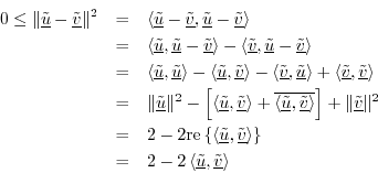
We can quickly show this for real vectors
![]() ,
,
![]() , as
follows: If either
, as
follows: If either
![]() or
or
![]() is zero, the inequality holds (as
equality). Assuming both are nonzero, let's scale them to unit-length
by defining the normalized vectors
is zero, the inequality holds (as
equality). Assuming both are nonzero, let's scale them to unit-length
by defining the normalized vectors
![]() ,
,
![]() , which are
unit-length vectors lying on the ``unit ball'' in
, which are
unit-length vectors lying on the ``unit ball'' in ![]() (a hypersphere
of radius
(a hypersphere
of radius ![]() ). We have
). We have
which implies
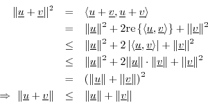
Triangle Inequality
The triangle inequality states that the length of any side of a
triangle is less than or equal to the sum of the lengths of the other two
sides, with equality occurring only when the triangle degenerates to a
line. In ![]() , this becomes
, this becomes
Triangle Difference Inequality
A useful variation on the triangle inequality is that the length of any side of a triangle is greater than the absolute difference of the lengths of the other two sides:
Proof: By the triangle inequality,
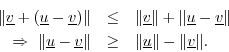
Interchanging
![]() and
and
![]() establishes the absolute value on the
right-hand side.
establishes the absolute value on the
right-hand side.
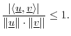
Vector Cosine
The Cauchy-Schwarz Inequality can be written
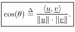
Orthogonality
The vectors (signals) ![]() and
and
![]() 5.11are said to be orthogonal if
5.11are said to be orthogonal if
![]() , denoted
, denoted ![]() .
That is to say
.
That is to say
Note that if ![]() and
and ![]() are real and orthogonal, the cosine of the angle
between them is zero. In plane geometry (
are real and orthogonal, the cosine of the angle
between them is zero. In plane geometry (![]() ), the angle between two
perpendicular lines is
), the angle between two
perpendicular lines is ![]() , and
, and
![]() , as expected. More
generally, orthogonality corresponds to the fact that two vectors in
, as expected. More
generally, orthogonality corresponds to the fact that two vectors in
![]() -space intersect at a right angle and are thus perpendicular
geometrically.
-space intersect at a right angle and are thus perpendicular
geometrically.
Example (![]() ):
):
Let ![]() and
and ![]() , as shown in Fig.5.8.
, as shown in Fig.5.8.
![\includegraphics[scale=0.7]{eps/ip}](http://www.dsprelated.com/josimages_new/mdft/img856.png)
The inner product is
![]() .
This shows that the vectors are orthogonal. As marked in the figure,
the lines intersect at a right angle and are therefore perpendicular.
.
This shows that the vectors are orthogonal. As marked in the figure,
the lines intersect at a right angle and are therefore perpendicular.
The Pythagorean Theorem in N-Space
In 2D, the Pythagorean Theorem says that when ![]() and
and ![]() are
orthogonal, as in Fig.5.8, (i.e., when the vectors
are
orthogonal, as in Fig.5.8, (i.e., when the vectors ![]() and
and ![]() intersect at a right angle), then we have
intersect at a right angle), then we have
This relationship generalizes to
If
Note that the converse is not true in ![]() . That is,
. That is,
![]() does not imply
does not imply
![]() in
in ![]() . For a counterexample, consider
. For a counterexample, consider ![]() ,
,
![]() , in which case
, in which case
For real vectors
![]() , the Pythagorean theorem Eq.
, the Pythagorean theorem Eq.![]() (5.1)
holds if and only if the vectors are orthogonal. To see this, note
that, from Eq.
(5.1)
holds if and only if the vectors are orthogonal. To see this, note
that, from Eq.![]() (5.2), when the Pythagorean theorem holds, either
(5.2), when the Pythagorean theorem holds, either
![]() or
or ![]() is zero, or
is zero, or
![]() is zero or purely imaginary,
by property 1 of norms (see §5.8.2). If the inner product
cannot be imaginary, it must be zero.
is zero or purely imaginary,
by property 1 of norms (see §5.8.2). If the inner product
cannot be imaginary, it must be zero.
Note that we also have an alternate version of the Pythagorean theorem:
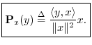
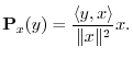
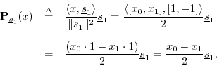
Projection
The orthogonal projection (or simply ``projection'') of
![]() onto
onto
![]() is defined by
is defined by
Motivation: The basic idea of orthogonal projection of ![]() onto
onto
![]() is to ``drop a perpendicular'' from
is to ``drop a perpendicular'' from ![]() onto
onto ![]() to define a new
vector along
to define a new
vector along ![]() which we call the ``projection'' of
which we call the ``projection'' of ![]() onto
onto ![]() .
This is illustrated for
.
This is illustrated for ![]() in Fig.5.9 for
in Fig.5.9 for ![]() and
and
![]() , in which case
, in which case
![$\displaystyle {\bf P}_{x}(y) \isdef \frac{\left<y,x\right>}{\Vert x\Vert^2} x
...
...{1})}{4^2+1^2} x
= \frac{11}{17} x= \left[\frac{44}{17},\frac{11}{17}\right].
$](http://www.dsprelated.com/josimages_new/mdft/img880.png)
![\includegraphics[scale=0.7]{eps/proj}](http://www.dsprelated.com/josimages_new/mdft/img881.png)
Derivation: (1) Since any projection onto ![]() must lie along the
line collinear with
must lie along the
line collinear with ![]() , write the projection as
, write the projection as
![]() . (2) Since by definition the projection error
. (2) Since by definition the projection error
![]() is orthogonal to
is orthogonal to ![]() , we must have
, we must have
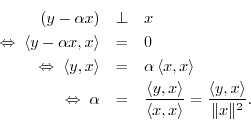
Thus,
See §I.3.3 for illustration of orthogonal projection in matlab.
Signal Reconstruction from Projections
We now know how to project a signal onto other signals. We now need
to learn how to reconstruct a signal
![]() from its projections
onto
from its projections
onto ![]() different vectors
different vectors
![]() ,
,
![]() . This
will give us the inverse DFT operation (or the inverse of
whatever transform we are working with).
. This
will give us the inverse DFT operation (or the inverse of
whatever transform we are working with).
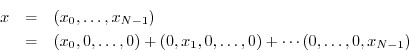
As a simple example, consider the projection of a signal
![]() onto the
rectilinear coordinate axes of
onto the
rectilinear coordinate axes of ![]() . The coordinates of the
projection onto the 0th coordinate axis are simply
. The coordinates of the
projection onto the 0th coordinate axis are simply
![]() .
The projection along coordinate axis
.
The projection along coordinate axis ![]() has coordinates
has coordinates
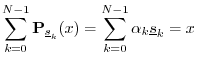
![]() , and so on. The original signal
, and so on. The original signal ![]() is then clearly
the vector sum of its projections onto the coordinate axes:
is then clearly
the vector sum of its projections onto the coordinate axes:
To make sure the previous paragraph is understood, let's look at the
details for the case ![]() . We want to project an arbitrary
two-sample signal
. We want to project an arbitrary
two-sample signal
![]() onto the coordinate axes in 2D. A
coordinate axis can be generated by multiplying any nonzero vector by
scalars. The horizontal axis can be represented by any vector of the
form
onto the coordinate axes in 2D. A
coordinate axis can be generated by multiplying any nonzero vector by
scalars. The horizontal axis can be represented by any vector of the
form
![]() ,
,
![]() while the vertical axis can be
represented by any vector of the form
while the vertical axis can be
represented by any vector of the form
![]() ,
,
![]() .
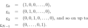
For maximum simplicity, let's choose
.
For maximum simplicity, let's choose
![\begin{eqnarray*}
\underline{e}_0 &\isdef & [1,0], \\
\underline{e}_1 &\isdef & [0,1].
\end{eqnarray*}](http://www.dsprelated.com/josimages_new/mdft/img895.png)
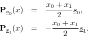
The projection of ![]() onto
onto
![]() is, by definition,
is, by definition,
![\begin{eqnarray*}
{\bf P}_{\underline{e}_0}(x) &\isdef & \frac{\left<x,\underlin...
...0}) \underline{e}_0
= x_0 \underline{e}_0\\ [5pt]
&=& [x_0,0].
\end{eqnarray*}](http://www.dsprelated.com/josimages_new/mdft/img897.png)
Similarly, the projection of ![]() onto
onto
![]() is
is
![\begin{eqnarray*}
{\bf P}_{\underline{e}_1}(x) &\isdef & \frac{\left<x,\underlin...
...1}) \underline{e}_1
= x_1 \underline{e}_1\\ [5pt]
&=& [0,x_1].
\end{eqnarray*}](http://www.dsprelated.com/josimages_new/mdft/img899.png)
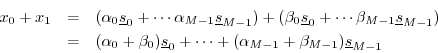
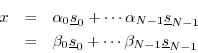
The reconstruction of ![]() from its projections onto the coordinate
axes is then the vector sum of the projections:
from its projections onto the coordinate
axes is then the vector sum of the projections:
The projection of a vector onto its coordinate axes is in some sense
trivial because the very meaning of the coordinates is that they are
scalars ![]() to be applied to the coordinate vectors
to be applied to the coordinate vectors
![]() in
order to form an arbitrary vector
in
order to form an arbitrary vector
![]() as a linear combination
of the coordinate vectors:
as a linear combination
of the coordinate vectors:
Changing Coordinates
What's more interesting is when we project a signal ![]() onto a set
of vectors other than the coordinate set. This can be viewed
as a change of coordinates in
onto a set
of vectors other than the coordinate set. This can be viewed
as a change of coordinates in ![]() . In the case of the DFT,
the new vectors will be chosen to be sampled complex sinusoids.
. In the case of the DFT,
the new vectors will be chosen to be sampled complex sinusoids.
An Example of Changing Coordinates in 2D
As a simple example, let's pick the following pair of new coordinate vectors in 2D:
![\begin{eqnarray*}
\sv_0 &\isdef & [1,1] \\
\sv_1 &\isdef & [1,-1]
\end{eqnarray*}](http://www.dsprelated.com/josimages_new/mdft/img905.png)
These happen to be the DFT sinusoids for ![]() having frequencies
having frequencies ![]() (``dc'') and
(``dc'') and ![]() (half the sampling rate). (The sampled complex
sinusoids of the DFT reduce to real numbers only for
(half the sampling rate). (The sampled complex
sinusoids of the DFT reduce to real numbers only for ![]() and
and ![]() .) We
already showed in an earlier example that these vectors are orthogonal. However, they are not orthonormal since the norm is
.) We
already showed in an earlier example that these vectors are orthogonal. However, they are not orthonormal since the norm is
![]() in each case. Let's try projecting
in each case. Let's try projecting ![]() onto these vectors and
seeing if we can reconstruct by summing the projections.
onto these vectors and
seeing if we can reconstruct by summing the projections.
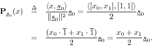
The projection of ![]() onto
onto ![]() is, by
definition,5.12
is, by
definition,5.12
Similarly, the projection of ![]() onto
onto ![]() is
is
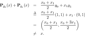
The sum of these projections is then
![\begin{eqnarray*}
{\bf P}_{\sv_0}(x) + {\bf P}_{\sv_1}(x) &=&
\frac{x_0 + x_1}...
...} - \frac{x_0 - x_1}{2}\right) \\ [5pt]
&=& (x_0,x_1) \isdef x.
\end{eqnarray*}](http://www.dsprelated.com/josimages_new/mdft/img915.png)
It worked!
Projection onto Linearly Dependent Vectors
Now consider another example:
![\begin{eqnarray*}
\sv_0 &\isdef & [1,1], \\
\sv_1 &\isdef & [-1,-1].
\end{eqnarray*}](http://www.dsprelated.com/josimages_new/mdft/img916.png)
The projections of
![]() onto these vectors are
onto these vectors are
The sum of the projections is
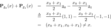
Something went wrong, but what? It turns out that a set of ![]() vectors can be used to reconstruct an arbitrary vector in
vectors can be used to reconstruct an arbitrary vector in ![]() from
its projections only if they are linearly independent. In
general, a set of vectors is linearly independent if none of them can
be expressed as a linear combination of the others in the set. What
this means intuitively is that they must ``point in different
directions'' in
from
its projections only if they are linearly independent. In
general, a set of vectors is linearly independent if none of them can
be expressed as a linear combination of the others in the set. What
this means intuitively is that they must ``point in different
directions'' in ![]() -space. In this example
-space. In this example
![]() so that they
lie along the same line in
so that they
lie along the same line in ![]() -space. As a result, they are
linearly dependent: one is a linear combination of the other
(
-space. As a result, they are
linearly dependent: one is a linear combination of the other
(
![]() ).
).
Projection onto Non-Orthogonal Vectors
Consider this example:
![\begin{eqnarray*}
\sv_0 &\isdef & [1,1] \\
\sv_1 &\isdef & [0,1]
\end{eqnarray*}](http://www.dsprelated.com/josimages_new/mdft/img922.png)
These point in different directions, but they are not orthogonal. What happens now? The projections are
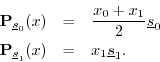
The sum of the projections is
So, even though the vectors are linearly independent, the sum of
projections onto them does not reconstruct the original vector. Since the
sum of projections worked in the orthogonal case, and since orthogonality
implies linear independence, we might conjecture at this point that the sum
of projections onto a set of ![]() vectors will reconstruct the original
vector only when the vector set is orthogonal, and this is true,
as we will show.
vectors will reconstruct the original
vector only when the vector set is orthogonal, and this is true,
as we will show.
It turns out that one can apply an orthogonalizing process, called
Gram-Schmidt orthogonalization to any ![]() linearly independent
vectors in
linearly independent
vectors in ![]() so as to form an orthogonal set which will always
work. This will be derived in Section 5.10.4.
so as to form an orthogonal set which will always
work. This will be derived in Section 5.10.4.
Obviously, there must be at least ![]() vectors in the set. Otherwise,
there would be too few degrees of freedom to represent an
arbitrary
vectors in the set. Otherwise,
there would be too few degrees of freedom to represent an
arbitrary
![]() . That is, given the
. That is, given the ![]() coordinates
coordinates
![]() of
of ![]() (which are scale factors relative to
the coordinate vectors
(which are scale factors relative to
the coordinate vectors
![]() in
in ![]() ), we have to find at least
), we have to find at least ![]() coefficients of projection (which we may think of as coordinates
relative to new coordinate vectors
coefficients of projection (which we may think of as coordinates
relative to new coordinate vectors ![]() ). If we compute only
). If we compute only ![]() coefficients, then we would be mapping a set of
coefficients, then we would be mapping a set of ![]() complex numbers to
complex numbers to
![]() numbers. Such a mapping cannot be invertible in general. It
also turns out
numbers. Such a mapping cannot be invertible in general. It
also turns out ![]() linearly independent vectors is always sufficient.
The next section will summarize the general results along these lines.
linearly independent vectors is always sufficient.
The next section will summarize the general results along these lines.
General Conditions
This section summarizes and extends the above derivations in a more
formal manner (following portions of chapter 4 of
![]() ). In
particular, we establish that the sum of projections of
). In
particular, we establish that the sum of projections of
![]() onto
onto ![]() vectors
vectors
![]() will give back the original vector
will give back the original vector
![]() whenever the set
whenever the set
![]() is an orthogonal
basis for
is an orthogonal
basis for ![]() .
.
Definition: A set of vectors is said to form a vector space if, given
any two members ![]() and
and ![]() from the set, the vectors
from the set, the vectors
![]() and
and ![]() are also in the set, where
are also in the set, where
![]() is any
scalar.
is any
scalar.
Definition: The set of all ![]() -dimensional complex vectors is denoted
-dimensional complex vectors is denoted
![]() . That is,
. That is, ![]() consists of all vectors
consists of all vectors
![]() defined as a list of
defined as a list of ![]() complex numbers
complex numbers
![]() .
.
Theorem: ![]() is a vector space under elementwise addition and
multiplication by complex scalars.
is a vector space under elementwise addition and
multiplication by complex scalars.
Proof: This is a special case of the following more general theorem.
Theorem: Let ![]() be an integer greater than 0. Then the set of all
linear combinations of
be an integer greater than 0. Then the set of all
linear combinations of ![]() vectors from
vectors from ![]() forms a vector space
under elementwise addition and multiplication by complex scalars.
forms a vector space
under elementwise addition and multiplication by complex scalars.
Proof: Let the original set of ![]() vectors be denoted
vectors be denoted
![]() .
Form
.
Form
which is yet another linear combination of the original vectors (since
complex numbers are closed under addition). Since we have shown that
scalar multiples and vector sums of linear combinations of the original
![]() vectors from
vectors from ![]() are also linear combinations of those same
original
are also linear combinations of those same
original ![]() vectors from
vectors from ![]() , we have that the defining properties
of a vector space are satisfied.
, we have that the defining properties
of a vector space are satisfied.
![]()
Note that the closure of vector addition and scalar multiplication are ``inherited'' from the closure of complex numbers under addition and multiplication.
Corollary: The set of all linear combinations of ![]() real vectors
real vectors
![]() , using real scalars
, using real scalars
![]() , form a
vector space.
, form a
vector space.
Definition: The set of all linear combinations of a set of ![]() complex vectors from
complex vectors from ![]() , using complex scalars, is called a
complex vector space of dimension
, using complex scalars, is called a
complex vector space of dimension ![]() .
.
Definition: The set of all linear combinations of a set of ![]() real vectors
from
real vectors
from ![]() , using real scalars, is called a real vector
space of dimension
, using real scalars, is called a real vector
space of dimension ![]() .
.
Definition: If a vector space consists of the set of all linear
combinations of a finite set of vectors
![]() , then
those vectors are said to span the space.
, then
those vectors are said to span the space.
Example: The coordinate vectors in ![]() span
span ![]() since every vector
since every vector
![]() can be expressed as a linear combination of the coordinate vectors
as
can be expressed as a linear combination of the coordinate vectors
as
Definition: The vector space spanned by a set of ![]() vectors from
vectors from ![]() is called an
is called an ![]() -dimensional subspace of
-dimensional subspace of ![]() .
.
Definition: A vector
![]() is said to be linearly dependent on
a set of
is said to be linearly dependent on
a set of ![]() vectors
vectors
![]() ,
,
![]() , if
, if
![]() can be expressed as a linear combination of those
can be expressed as a linear combination of those ![]() vectors.
vectors.
Thus,
![]() is linearly dependent on
is linearly dependent on
![]() if there
exist scalars
if there
exist scalars
![]() such that
such that
![]() . Note that the zero vector
is linearly dependent on every collection of vectors.
. Note that the zero vector
is linearly dependent on every collection of vectors.
Theorem: (i) If
![]() span a vector space, and if one of them,
say
span a vector space, and if one of them,
say ![]() , is linearly dependent on the others, then the same vector
space is spanned by the set obtained by omitting
, is linearly dependent on the others, then the same vector
space is spanned by the set obtained by omitting ![]() from the
original set. (ii) If
from the
original set. (ii) If
![]() span a vector space,
we can always select from these a linearly independent set that spans
the same space.
span a vector space,
we can always select from these a linearly independent set that spans
the same space.
Proof: Any ![]() in the space can be represented as a linear combination of the
vectors
in the space can be represented as a linear combination of the
vectors
![]() . By expressing
. By expressing ![]() as a linear
combination of the other vectors in the set, the linear combination
for
as a linear
combination of the other vectors in the set, the linear combination
for ![]() becomes a linear combination of vectors other than
becomes a linear combination of vectors other than ![]() .
Thus,
.
Thus, ![]() can be eliminated from the set, proving (i). To prove
(ii), we can define a procedure for forming the required subset of the
original vectors: First, assign
can be eliminated from the set, proving (i). To prove
(ii), we can define a procedure for forming the required subset of the
original vectors: First, assign ![]() to the set. Next, check to
see if
to the set. Next, check to
see if ![]() and
and ![]() are linearly dependent. If so (i.e.,
are linearly dependent. If so (i.e.,
![]() is a scalar times
is a scalar times ![]() ), then discard
), then discard ![]() ; otherwise
assign it also to the new set. Next, check to see if
; otherwise
assign it also to the new set. Next, check to see if ![]() is
linearly dependent on the vectors in the new set. If it is (i.e.,
is
linearly dependent on the vectors in the new set. If it is (i.e.,
![]() is some linear combination of
is some linear combination of ![]() and
and ![]() ) then
discard it; otherwise assign it also to the new set. When this
procedure terminates after processing
) then
discard it; otherwise assign it also to the new set. When this
procedure terminates after processing ![]() , the new set will
contain only linearly independent vectors which span the original
space.
, the new set will
contain only linearly independent vectors which span the original
space.
Definition: A set of linearly independent vectors which spans a vector space
is called a basis for that vector space.
Definition: The set of coordinate vectors in ![]() is called the natural basis for
is called the natural basis for ![]() , where the
, where the ![]() th basis vector
is
th basis vector
is
![$\displaystyle \underline{e}_n = [\;0\;\;\cdots\;\;0\;\underbrace{1}_{\mbox{$n$th}}\;\;0\;\;\cdots\;\;0].
$](http://www.dsprelated.com/josimages_new/mdft/img955.png)
Theorem: The linear combination expressing a vector in terms of basis vectors
for a vector space is unique.
Proof: Suppose a vector
![]() can be expressed in two different ways as
a linear combination of basis vectors
can be expressed in two different ways as
a linear combination of basis vectors
![]() :
:
where
![]() for at least one value of
for at least one value of
![]() .
Subtracting the two representations gives
.
Subtracting the two representations gives
Note that while the linear combination relative to a particular basis is
unique, the choice of basis vectors is not. For example, given any basis
set in ![]() , a new basis can be formed by rotating all vectors in
, a new basis can be formed by rotating all vectors in
![]() by the same angle. In this way, an infinite number of basis sets can
be generated.
by the same angle. In this way, an infinite number of basis sets can
be generated.
As we will soon show, the DFT can be viewed as a change of
coordinates from coordinates relative to the natural basis in ![]() ,
,
![]() , to coordinates relative to the sinusoidal
basis for
, to coordinates relative to the sinusoidal
basis for ![]() ,
,
![]() , where
, where
![]() . The sinusoidal basis set for
. The sinusoidal basis set for ![]() consists of length
consists of length
![]() sampled complex sinusoids at frequencies
sampled complex sinusoids at frequencies
![]() . Any scaling of these vectors in
. Any scaling of these vectors in ![]() by complex
scale factors could also be chosen as the sinusoidal basis (i.e., any
nonzero amplitude and any phase will do). However, for simplicity, we will
only use unit-amplitude, zero-phase complex sinusoids as the Fourier
``frequency-domain'' basis set. To summarize this paragraph, the
time-domain samples of a signal are its coordinates relative to the natural
basis for
by complex
scale factors could also be chosen as the sinusoidal basis (i.e., any
nonzero amplitude and any phase will do). However, for simplicity, we will
only use unit-amplitude, zero-phase complex sinusoids as the Fourier
``frequency-domain'' basis set. To summarize this paragraph, the
time-domain samples of a signal are its coordinates relative to the natural
basis for ![]() , while its spectral coefficients are the coordinates of the
signal relative to the sinusoidal basis for
, while its spectral coefficients are the coordinates of the
signal relative to the sinusoidal basis for ![]() .
.
Theorem: Any two bases of a vector space contain the same number of vectors.
Proof: Left as an exercise (or see [47]).
Definition: The number of vectors in a basis for a particular space is called
the dimension of the space. If the dimension is ![]() , the space is
said to be an
, the space is
said to be an ![]() dimensional space, or
dimensional space, or ![]() -space.
-space.
In this book, we will only consider finite-dimensional vector spaces in any detail. However, the discrete-time Fourier transform (DTFT) and Fourier transform (FT) both require infinite-dimensional basis sets, because there is an infinite number of points in both the time and frequency domains. (See Appendix B for details regarding the FT and DTFT.)
Signal/Vector Reconstruction from Projections
We now arrive finally at the main desired result for this section:
Theorem: The projections of any vector
![]() onto any orthogonal basis set
for
onto any orthogonal basis set
for ![]() can be summed to reconstruct
can be summed to reconstruct ![]() exactly.
exactly.
Proof: Let
![]() denote any orthogonal basis set for
denote any orthogonal basis set for ![]() .
Then since
.
Then since ![]() is in the space spanned by these vectors, we have
is in the space spanned by these vectors, we have
for some (unique) scalars
![$\displaystyle {\bf P}_{\sv_k}(\sv_l) \isdef
\frac{\left<\sv_l,\sv_k\right>}{\l...
...ll}
\underline{0}, & l\neq k \\ [5pt]
\sv_k, & l=k. \\
\end{array} \right.
$](http://www.dsprelated.com/josimages_new/mdft/img973.png)
Gram-Schmidt Orthogonalization
Recall from the end of §5.10 above that an
orthonormal set of vectors is a set of unit-length
vectors that are mutually orthogonal. In other words,
orthonormal vector set is just an orthogonal vector set in which each
vector ![]() has been normalized to unit length
has been normalized to unit length
![]() .
.
Theorem: Given a set of ![]() linearly independent vectors
linearly independent vectors
![]() from
from ![]() , we can construct an
orthonormal set
, we can construct an
orthonormal set
![]() which are linear
combinations of the original set and which span the same space.
which are linear
combinations of the original set and which span the same space.
Proof: We prove the theorem by constructing the desired orthonormal
set
![]() sequentially from the original set
sequentially from the original set ![]() .
This procedure is known as Gram-Schmidt orthogonalization.
.
This procedure is known as Gram-Schmidt orthogonalization.
First, note that
![]() for all
for all ![]() , since
, since
![]() is
linearly dependent on every vector. Therefore,
is
linearly dependent on every vector. Therefore,
![]() .
.
- Set
 .
.
- Define
 as
as  minus the projection of
onto
minus the projection of
onto
 :
The vector
:
The vector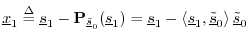 is orthogonal to
by construction. (We
subtracted out the part of that wasn't orthogonal to
.) Also, since and
is orthogonal to
by construction. (We
subtracted out the part of that wasn't orthogonal to
.) Also, since and  are linearly independent,
we have
are linearly independent,
we have
 .
.
- Set
 (i.e., normalize the result
of the preceding step).
(i.e., normalize the result
of the preceding step).
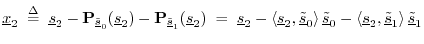
- Define
 as
as  minus the projection of
onto
and
minus the projection of
onto
and
 :
:
- Normalize:
 .
.
- Continue this process until
 has been defined.
The Gram-Schmidt orthogonalization procedure will construct an
orthonormal basis from any set of ![]() linearly independent vectors.
Obviously, by skipping the normalization step, we could also form
simply an orthogonal basis. The key ingredient of this procedure is
that each new basis vector is obtained by subtracting out the
projection of the next linearly independent vector onto the vectors
accepted so far into the set. We may say that each new linearly
independent vector
linearly independent vectors.
Obviously, by skipping the normalization step, we could also form
simply an orthogonal basis. The key ingredient of this procedure is
that each new basis vector is obtained by subtracting out the
projection of the next linearly independent vector onto the vectors
accepted so far into the set. We may say that each new linearly
independent vector ![]() is projected onto the subspace
spanned by the vectors
is projected onto the subspace
spanned by the vectors
![]() , and any nonzero
projection in that subspace is subtracted out of
, and any nonzero
projection in that subspace is subtracted out of ![]() to make the
new vector orthogonal to the entire subspace. In other words, we
retain only that portion of each new vector
to make the
new vector orthogonal to the entire subspace. In other words, we
retain only that portion of each new vector ![]() which ``points
along'' a new dimension. The first direction is arbitrary and is
determined by whatever vector we choose first (
which ``points
along'' a new dimension. The first direction is arbitrary and is
determined by whatever vector we choose first (![]() here). The
next vector is forced to be orthogonal to the first. The second is
forced to be orthogonal to the first two (and thus to the 2D subspace
spanned by them), and so on.
here). The
next vector is forced to be orthogonal to the first. The second is
forced to be orthogonal to the first two (and thus to the 2D subspace
spanned by them), and so on.
This chapter can be considered an introduction to some important concepts of linear algebra. The student is invited to pursue further reading in any textbook on linear algebra, such as [47].5.13
Matlab/Octave examples related to this chapter appear in Appendix I.
Signal Projection Problems
See http://ccrma.stanford.edu/~jos/mdftp/Signal_Projection_Problems.html
Next Section:
Derivation of the Discrete Fourier Transform (DFT)
Previous Section:
Sinusoids and Exponentials


