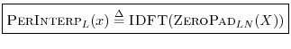
The dual of the zero-padding theorem states formally that
zero padding in the frequency domain corresponds to periodic
interpolation in the time domain:
Definition: For all
 and any integer
  ,
,
 |
(7.7) |
where zero padding is defined in §
7.2.7 and illustrated in
Figure
7.7. In other words, zero-padding a
DFT by the factor

in
the frequency domain
(by inserting

zeros at
bin number 
corresponding to
the
folding frequency7.21)
gives rise to ``periodic interpolation'' by the factor
in the time
domain. It is straightforward to show that the interpolation kernel
used in periodic interpolation is an
aliased sinc function,
that is, a
sinc function
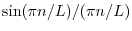
that has been
time-
aliased on a block of length

. Such an
aliased sinc function
is of course periodic with
period samples. See Appendix
D
for a discussion of
ideal bandlimited interpolation, in which
the interpolating
sinc function is not aliased.
Periodic interpolation is ideal for signals that are periodic
in  samples, where is the DFT length. For non-periodic
signals, which is almost always the case in practice, bandlimited
interpolation should be used instead (Appendix D).
samples, where is the DFT length. For non-periodic
signals, which is almost always the case in practice, bandlimited
interpolation should be used instead (Appendix D).
It is instructive to interpret the periodic interpolation theorem in
terms of the stretch theorem,
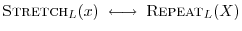 .
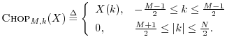
To do this, it is convenient to define a ``zero-centered rectangular
window'' operator:
.
To do this, it is convenient to define a ``zero-centered rectangular
window'' operator:
Definition: For any
 and any odd integer
  we define the
length
we define the
length  even rectangular windowing operation by
Thus, this ``
zero-phase rectangular window,'' when applied to a
spectrum 
, sets the
spectrum to zero everywhere outside a
zero-centered interval of
samples. Note that

is
the
ideal lowpass filtering operation in the frequency domain.
The ``cut-off frequency'' is
![$ \omega_c = 2\pi[(M-1)/2]/N$](http://www.dsprelated.com/josimages_new/mdft/img1463.png)
radians per
sample.
For even
, we allow

to be ``passed'' by the window,
but in our usage (below), this sample should always be zero anyway.
With this notation defined we can efficiently restate
periodic interpolation in terms of the

operator:
Theorem: When
consists of one or more periods from a periodic
signal
 ,
,
In other words, ideal periodic interpolation of one period of

by
the integer factor
may be carried out by first stretching
by
the factor
(inserting

zeros between adjacent samples of
), taking the
DFT, applying the ideal
lowpass filter as an
-point rectangular window in the frequency domain, and performing
the inverse DFT.
Proof: First, recall that
 . That is,
stretching a signal by the factor gives a new signal
. That is,
stretching a signal by the factor gives a new signal
 which has a spectrum
  consisting of copies of
repeated around the unit circle. The ``baseband copy'' of in
can be defined as the -sample sequence centered about frequency
zero. Therefore, we can use an ``ideal filter'' to ``pass'' the
baseband spectral copy and zero out all others, thereby converting
consisting of copies of
repeated around the unit circle. The ``baseband copy'' of in
can be defined as the -sample sequence centered about frequency
zero. Therefore, we can use an ``ideal filter'' to ``pass'' the
baseband spectral copy and zero out all others, thereby converting
 to
to
 . I.e.,
The last step is provided by the
zero-padding theorem (§
7.4.12).
The previous result can be extended toward bandlimited interpolation
of
 which includes all nonzero samples from an
arbitrary time-limited signal
(i.e., going beyond the interpolation of only periodic bandlimited
signals given one or more periods
) by
which includes all nonzero samples from an
arbitrary time-limited signal
(i.e., going beyond the interpolation of only periodic bandlimited
signals given one or more periods
) by
- replacing the rectangular window
 with a
smoother spectral window
with a
smoother spectral window  , and
, and
- using extra zero-padding in the time domain to convert the
cyclic convolution between
 and
and  into an
acyclic convolution between them (recall §7.2.4).
into an
acyclic convolution between them (recall §7.2.4).
The smoother spectral window

can be thought of as the
frequency response of the FIR
7.22 filter used as the
bandlimited interpolation kernel in the time domain. The number of
zeros needed in the zero-padding of
in the time domain is simply
length of
minus 1, and the number of zeros to be appended to
is the length of
minus 1. With this much
zero-padding, the
cyclic convolution of
and
implemented using
the
DFT becomes equivalent to acyclic convolution, as desired for the
time-limited signals
and
. Thus, if

denotes the nonzero
length of
, then the nonzero length of
is

, and we require the DFT length to be

, where

is the filter length. In operator
notation, we can express bandlimited
sampling-rate up-conversion by
the factor
for time-limited signals
by
 |
(7.8) |
The approximation symbol `

' approaches equality as the
spectral window
approaches
![$ \hbox{\sc Chop}_{N_x}([1,\dots,1])$](http://www.dsprelated.com/josimages_new/mdft/img1484.png)
(the
frequency response of the ideal
lowpass filter passing only the
original
spectrum ), while at the same time allowing no time
aliasing (convolution remains acyclic in the time domain).
Equation (7.8) can provide the basis for a high-quality
sampling-rate conversion algorithm. Arbitrarily long signals can be
accommodated by breaking them into segments of length , applying
the above algorithm to each block, and summing the up-sampled blocks using
overlap-add. That is, the lowpass filter ``rings''
into the next block and possibly beyond (or even into both adjacent
time blocks when is not causal), and this ringing must be summed
into all affected adjacent blocks. Finally, the filter can
``window away'' more than the top copies of in , thereby
preparing the time-domain signal for downsampling, say by
 :
:
where now the lowpass filter frequency response
must be close to
zero for all
. While such a
sampling-rate conversion algorithm can be made more efficient by using
an
FFT in place of the DFT (see Appendix
A), it is not necessarily
the most efficient algorithm possible. This is because (1)

out
of
output samples from the IDFT need not be computed at all, and
(2)
has many zeros in it which do not need explicit
handling. For an introduction to time-domain sampling-rate
conversion (bandlimited interpolation) algorithms which take advantage
of points (1) and (2) in this paragraph, see,
e.g., Appendix
D and
[
72].
Next Section: Why a DFT is usually called an FFT in practicePrevious Section: Zero Padding Theorem (Spectral Interpolation)