


Bowed Strings
A schematic block diagram for bowed strings is shown in Fig.9.51 [431]. The bow divides the string into two sections, so the bow model is a nonlinear two-port, in contrast with the reed which was a nonlinear one-port terminating the bore at the mouthpiece. In the case of bowed strings, the primary control variable is bow velocity, so velocity waves are the natural choice for the delay lines.
![\includegraphics[width=\twidth]{eps/fBowedStrings}](http://www.dsprelated.com/josimages_new/pasp/img2556.png)
Digital Waveguide Bowed-String
A more detailed diagram of the digital waveguide implementation of the
bowed-string instrument model is shown in Fig.9.52.
The right delay-line pair carries left-going and right-going velocity waves
samples
![]() and
and
![]() , respectively, which sample the traveling-wave
components within the string to the right of the bow, and similarly for the
section of string to the left of the bow. The `
, respectively, which sample the traveling-wave
components within the string to the right of the bow, and similarly for the
section of string to the left of the bow. The `![]() ' superscript refers to
waves traveling into the bow.
' superscript refers to
waves traveling into the bow.
![\includegraphics[width=\twidth]{eps/fBowedStringsWGM}](http://www.dsprelated.com/josimages_new/pasp/img2559.png)
String velocity at any point is obtained by adding a left-going
velocity sample to the right-going velocity sample immediately
opposite in the other delay line, as indicated in
Fig.9.52 at the bowing point. The reflection
filter at the right implements the losses at the bridge, bow, nut or
finger-terminations (when stopped), and the round-trip
attenuation/dispersion from traveling back and forth on the string. To
a very good degree of approximation, the nut reflects incoming
velocity waves (with a sign inversion) at all audio wavelengths. The
bridge behaves similarly to a first order, but there are additional
(complex) losses due to the finite bridge driving-point impedance
(necessary for transducing sound from the string into the resonating
body). According to [95, page 27], the bridge of a
violin can be modeled up to about ![]() kHz, for purposes of computing
string loss, as a single spring in parallel with a
frequency-independent resistance (``dashpot''). Bridge-filter
modeling is discussed further in §9.2.1.
kHz, for purposes of computing
string loss, as a single spring in parallel with a
frequency-independent resistance (``dashpot''). Bridge-filter
modeling is discussed further in §9.2.1.
Figure 9.52 is drawn for the case of the lowest
note. For higher notes the delay lines between the bow and nut are
shortened according to the distance between the bow and the finger
termination. The bow-string interface is controlled by differential
velocity
![]() which is defined as the bow velocity minus the total
incoming string velocity. Other controls include bow force and angle which are changed by modifying the reflection-coefficient
which is defined as the bow velocity minus the total
incoming string velocity. Other controls include bow force and angle which are changed by modifying the reflection-coefficient
![]() . Bow position is changed by taking samples from one delay-line
pair and appending them to the other delay-line pair. Delay-line
interpolation can be used to provide continuous change of bow position
[267].
. Bow position is changed by taking samples from one delay-line
pair and appending them to the other delay-line pair. Delay-line
interpolation can be used to provide continuous change of bow position
[267].
The Bow-String Scattering Junction
The theory of bow-string interaction is described in
[95,151,244,307,308]. The basic
operation of the bow is to reconcile the nonlinear bow-string friction
curve ![]() with the string wave impedance
with the string wave impedance ![]() :
:
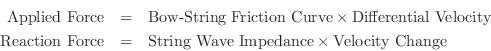
or, equating these equal and opposite forces, we obtain
![\includegraphics[width=4in]{eps/fBowFrictionCurve}](http://www.dsprelated.com/josimages_new/pasp/img2570.png) |
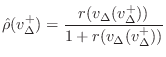
In a bowed string simulation as in Fig.9.51, a velocity input (which is injected equally in the left- and right-going directions) must be found such that the transverse force of the bow against the string is balanced by the reaction force of the moving string. If bow-hair dynamics are neglected [176], the bow-string interaction can be simulated using a memoryless table lookup or segmented polynomial in a manner similar to single-reed woodwinds [431].
A derivation analogous to that for the single reed is possible for the
simulation of the bow-string interaction. The final result is as follows.
where
Nominally,
![]() is constant (the so-called static coefficient
of friction) for
is constant (the so-called static coefficient
of friction) for
![]() , where
, where
![]() is both the
capture and break-away differential velocity. For
is both the
capture and break-away differential velocity. For
![]() ,
,
![]() falls quickly to a low dynamic coefficient of friction. It
is customary in the bowed-string physics literature to assume that the
dynamic coefficient of friction continues to approach zero with increasing
falls quickly to a low dynamic coefficient of friction. It
is customary in the bowed-string physics literature to assume that the
dynamic coefficient of friction continues to approach zero with increasing
![]() [308,95].
[308,95].
![\includegraphics[width=4in]{eps/fBowTable}](http://www.dsprelated.com/josimages_new/pasp/img2581.png)
Figure 9.54 illustrates a simplified, piecewise linear
bow table
![]() . The flat center portion corresponds to a
fixed reflection coefficient ``seen'' by a traveling wave encountering
the bow stuck against the string, and the outer sections of the curve
give a smaller reflection coefficient corresponding to the reduced
bow-string interaction force while the string is slipping under the
bow. The notation
. The flat center portion corresponds to a
fixed reflection coefficient ``seen'' by a traveling wave encountering
the bow stuck against the string, and the outer sections of the curve
give a smaller reflection coefficient corresponding to the reduced
bow-string interaction force while the string is slipping under the
bow. The notation
![]() at the corner point denotes the capture or
break-away differential velocity. Note that hysteresis is neglected.
at the corner point denotes the capture or
break-away differential velocity. Note that hysteresis is neglected.
Bowed String Synthesis Extensions
For maximally natural interaction between the bow and string, bow-hair dynamics should be included in a proper bow bodel [176]. In addition, the width of the bow should be variable, depending on bow ``angle''. A finite difference model for the finite width bow was reported in [351,352]. The bow-string friction characteristic should employ a thermodynamic model of bow friction in which the bow rosin has a time-varying viscosity due to temperature variations within a period of sound [549]. It is well known by bowed-string players that rosin is sensitive to temperature. Thermal models of dynamic friction in bowed strings are described in [426], and they have been used in virtual bowed strings for computer music [419,423,21].
Given a good model of a bowed-string instrument, it is most natural to interface it to a physical bow-type controller, with sensors for force, velocity, position, angle, and so on [420,294].
A real-time software implementation of a bowed-string model, similar to that shown in Fig.9.52, is available in the Synthesis Tool Kit (STK) distribution as Bowed.cpp. It provides a convenient starting point for more refined bowed-string models [276].
Linear Commuted Bowed Strings
The commuted synthesis technique (§8.7) can be extended to bowed strings in special case of ``ideal'' bowed attacks [440]. Here, an ideal attack is defined as one in which Helmholtz motion10.20is instantly achieved. This technique will be called ``linear commuted synthesis'' of bowed strings.
Additionally, the linear commuted-synthesis model for bowed strings can be driven by a separate nonlinear model of bowed-string dynamics. This gives the desirable combination of a full range of complex bow-string interaction behavior together with an efficiently implemented body resonator.
Bowing as Periodic Plucking
The ``leaning sawtooth'' waveforms observed by Helmholtz for steady state bowed strings can be obtained by periodically ``plucking'' the string in only one direction along the string [428]. In principle, a traveling impulsive excitation is introduced into the string in the right-going direction for a ``down bow'' and in the left-going direction for an ``up bow.'' This simplified bowing simulation works best for smooth bowing styles in which the notes have slow attacks. More varied types of attack can be achieved using the more physically accurate McIntyre-Woodhouse theory [307,431].
Commuting the string and resonator means that the string is now plucked by a periodically repeated resonator impulse response. A nice simplified vibrato implementation is available by varying the impulse-response retriggering period, i.e., the vibrato is implemented in the excitation oscillator and not in the delay loop. The string loop delay need not be modulated at all. While this departs from being a physical model, the vibrato quality is satisfying and qualitatively similar to that obtained by a rigorous physical model. Figure 9.55 illustrates the overall block diagram of the simplified bowed string and its commuted and response-excited versions.
![\includegraphics[width=\twidth]{eps/bowstringsbs}](http://www.dsprelated.com/josimages_new/pasp/img2583.png) |
In current technology, it is reasonable to store one recording of the resonator impulse response in digital memory as one of many possible string excitation tables. The excitation can contribute to many aspects of the tone to be synthesized, such as whether it is a violin or a cello, the force of the bow, and where the bow is playing on the string. Also, graphical equalization and other time-invariant filtering can be provided in the form of alternate excitation-table choices.
During the synthesis of a single bowed-string tone, the excitation signal is played into the string quasi-periodically. Since the excitation signal is typically longer than one period of the tone, it is necessary to either (1) interrupt the excitation playback to replay it from the beginning, or (2) start a new playback which overlaps with the playback in progress. Variant (2) requires a separate incrementing pointer and addition for each instance of the excitation playback; thus it is more expensive, but it is preferred from a quality standpoint. This same issue also arises in the Chant synthesis technique for the singing voice [389]. In the Chant technique, a sum of three or more enveloped sinusoids (called FOFs) is periodically played out to synthesize a sung vowel tone. In the unlikely event that the excitation table is less than one period long, it is of course extended by zeros, as is done in the VOSIM voice synthesis technique [219] which can be considered a simplified forerunner of Chant.
Sound examples for linear commuted bowed-string synthesis may be heard here: (WAV) (MP3) .
Of course, ordinary wavetable synthesis [303,199,327] or any other type of synthesis can also be used as an excitation signal in which case the string loop behaves as a pitch-synchronous comb filter following the wavetable oscillator. Interesting effects can be obtained by slightly detuning the wavetable oscillator and delay loop; tuning the wavetable oscillator to a harmonic of the delay loop can also produce an ethereal effect.
More General Quasi-Periodic Synthesis
![\includegraphics[width=\twidth]{eps/multiple_excitations}](http://www.dsprelated.com/josimages_new/pasp/img2584.png)
Figure 9.56 illustrates a more general version of the table-excited, filtered delay loop synthesis system [440]. The generalizations help to obtain a wider class of timbres. The multiple excitations summed together through time-varying gains provide for timbral evolution of the tone. For example, a violin can transform smoothly into a cello, or the bow can move smoothly toward the bridge by interpolating among two or more tables. Alternatively, the tables may contain ``principal components'' which can be scaled and added together to approximate a wider variety of excitation timbres. An excellent review of multiple wavetable synthesis appears in [199]. The nonlinearity is useful for obtaining distortion guitar sounds and other interesting evolving timbres [387].
Finally, the ``attack signal'' path around the string has been found to be useful for reducing the cost of implementation: the highest frequency components of a struck string, say, tend to emanate immediately from the string to the resonator with very little reflection back into the string (or pipe, in the case of wind instrument simulation). Injecting them into the delay loop increases the burden on the loop filter to quickly filter them out. Bypassing the delay loop altogether alleviates requirements on the loop filter and even allows the filtered delay loop to operate at a lower sampling rate; in this case, a signal interpolator would appear between the string output and the summer which adds in the scaled attack signal in Fig. 9.56. For example, it was found that the low E of an electric guitar (Gibson Les Paul) can be synthesized quite well using a filtered delay loop running at a sampling rate of 3 kHz. (The pickups do not pick up much energy above 1.5 kHz.) Similar savings can be obtained for any instrument having a high-frequency content which decays much more quickly than its low-frequency content.
Stochastic Excitation for Quasi-Periodic Synthesis
![\includegraphics[width=3.5in]{eps/noise_excitation}](http://www.dsprelated.com/josimages_new/pasp/img2585.png)
For good generality, at least one of the excitation signals should be a filtered noise signal [440]. An example implementation is shown in Fig. 9.57, in which there is a free-running bandlimited noise generator filtered by a finite impulse response (FIR) digital filter. As noted in §9.4.4, such a filtered-noise signal can synthesize the perceptual equivalent of the impulse response of many high-frequency modes that have been separated from the lower frequency modes in commuted synthesis (§8.7.1). It can also handle pluck models in which successive plucking variations are imposed by the FIR filter coefficients.
In a simple implementation, only two gains might be used, allowing simple interpolation from one filter to the next, and providing an overall amplitude control for the noise component of the excitation signal.
Next Section:
Brasses
Previous Section:
Woodwinds


