


Comb Filters
Comb filters are basic building blocks for digital audio effects. The acoustic echo simulation in Fig.2.9 is one instance of a comb filter. This section presents the two basic comb-filter types, feedforward and feedback, and gives a frequency-response analysis.
Feedforward Comb Filters
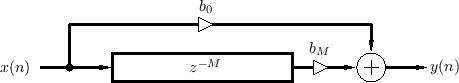
The feedforward comb filter is shown in Fig.2.23. The direct signal ``feeds forward'' around the delay line. The output is a linear combination of the direct and delayed signal.
The ``difference equation'' [449] for the feedforward comb filter is
We see that the feedforward comb filter is a particular type of FIR filter. It is also a special case of a TDL.
Note that the feedforward comb filter can implement the echo simulator
of Fig.2.9 by setting ![]() and
and ![]() . Thus, it is is a
computational physical model of a single discrete echo. This
is one of the simplest examples of acoustic modeling using signal
processing elements. The feedforward comb filter models the
superposition of a ``direct signal''
. Thus, it is is a
computational physical model of a single discrete echo. This
is one of the simplest examples of acoustic modeling using signal
processing elements. The feedforward comb filter models the
superposition of a ``direct signal'' ![]() plus an attenuated,
delayed signal
plus an attenuated,
delayed signal
![]() , where the attenuation (by
, where the attenuation (by ![]() ) is
due to ``air absorption'' and/or spherical spreading losses, and the
delay is due to acoustic propagation over the distance
) is
due to ``air absorption'' and/or spherical spreading losses, and the
delay is due to acoustic propagation over the distance ![]() meters,
where
meters,
where ![]() is the sampling period in seconds, and
is the sampling period in seconds, and ![]() is sound speed.
In cases where the simulated propagation delay needs to be more
accurate than the nearest integer number of samples
is sound speed.
In cases where the simulated propagation delay needs to be more
accurate than the nearest integer number of samples ![]() , some kind of
delay-line interpolation needs to be used (the subject of
§4.1). Similarly, when air absorption needs to be
simulated more accurately, the constant attenuation factor
, some kind of
delay-line interpolation needs to be used (the subject of
§4.1). Similarly, when air absorption needs to be
simulated more accurately, the constant attenuation factor ![]() can
be replaced by a linear, time-invariant filter
can
be replaced by a linear, time-invariant filter ![]() giving a
different attenuation at every frequency. Due to the physics of air
absorption,
giving a
different attenuation at every frequency. Due to the physics of air
absorption, ![]() is generally lowpass in character [349, p. 560], [47,318].
is generally lowpass in character [349, p. 560], [47,318].
Feedback Comb Filters
The feedback comb filter uses feedback instead of a feedforward signal, as shown in Fig.2.24 (drawn in ``direct form 2'' [449]).
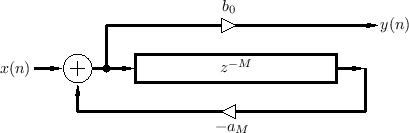
A difference equation describing the feedback comb filter can be written in ``direct form 1'' [449] as3.9
For stability, the feedback coefficient ![]() must be less than
must be less than
![]() in magnitude, i.e.,
in magnitude, i.e.,
![]() . Otherwise, if
. Otherwise, if
![]() ,
each echo will be louder than the previous echo, producing a
never-ending, growing series of echoes.
,
each echo will be louder than the previous echo, producing a
never-ending, growing series of echoes.
Sometimes the output signal is taken from the end of the delay line instead of the beginning, in which case the difference equation becomes
Feedforward Comb Filter Amplitude Response
Comb filters get their name from the ``comb-like'' appearance of their amplitude response (gain versus frequency), as shown in Figures 2.25, 2.26, and 2.27. For a review of frequency-domain analysis of digital filters, see, e.g., [449].
![\includegraphics[width=\twidth ]{eps/ffcfar}](http://www.dsprelated.com/josimages_new/pasp/img499.png) |
The transfer function of the feedforward comb filter Eq.![]() (2.2) is
(2.2) is
so that the amplitude response (gain versus frequency) is
This is plotted in Fig.2.25 for
Feedback Comb Filter Amplitude Response
Figure 2.26 shows a family of feedback-comb-filter amplitude responses, obtained using a selection of feedback coefficients.
![\includegraphics[width=\twidth ]{eps/fbcfar}](http://www.dsprelated.com/josimages_new/pasp/img505.png) |
Figure 2.27 shows a similar family obtained using negated feedback coefficients; the opposite sign of the feedback exchanges the peaks and valleys in the amplitude response.
![\includegraphics[width=\twidth ]{eps/fbcfiar}](http://www.dsprelated.com/josimages_new/pasp/img506.png) |
As introduced in §2.6.2 above, a class of feedback comb filters can be defined as any difference equation of the form
so that the amplitude response is
For ![]() , the feedback-comb amplitude response
reduces to
, the feedback-comb amplitude response
reduces to
Note that ![]() produces resonant peaks at
produces resonant peaks at
Filtered-Feedback Comb Filters
The filtered-feedback comb filter (FFBCF) uses filtered feedback instead of just a feedback gain.
Denoting the feedback-filter transfer function by ![]() , the
transfer function of the filtered-feedback comb filter can be written
as
, the
transfer function of the filtered-feedback comb filter can be written
as
In §2.6.2 above, we mentioned the physical interpretation of a feedback-comb-filter as simulating a plane-wave bouncing back and forth between two walls. Inserting a lowpass filter in the feedback loop further simulates frequency dependent losses incurred during a propagation round-trip, as naturally occurs in real rooms.
The main physical sources of plane-wave attenuation are air absorption (§B.7.15) and the coefficient of absorption at each wall [349]. Additional ``losses'' for plane waves in real rooms occur due to scattering. (The plane wave hits something other than a wall and reflects off in many different directions.) A particular scatterer used in concert halls is textured wall surfaces. In ray-tracing simulations, reflections from such walls are typically modeled as having a specular and diffuse component. Generally speaking, wavelengths that are large compared with the ``grain size'' of the wall texture reflect specularly (with some attenuation due to any wall motion), while wavelengths on the order of or smaller than the texture grain size are scattered in various directions, contributing to the diffuse component of reflection.
The filtered-feedback comb filter has many applications in computer music. It was evidently first suggested for artificial reverberation by Schroeder [412, p. 223], and first implemented by Moorer [314]. (Reverberation applications are discussed further in §3.6.) In the physical interpretation [428,207] of the Karplus-Strong algorithm [236,233], the FFBCF can be regarded as a transfer-function physical-model of a vibrating string. In digital waveguide modeling of string and wind instruments, FFBCFs are typically derived routinely as a computationally optimized equivalent forms based on some initial waveguide model developed in terms of bidirectional delay-lines (``digital waveguides'') (see §6.10.1 for an example).
For stability, the amplitude-response of the feedback-filter
![]() must be less than
must be less than ![]() in magnitude at all frequencies, i.e.,
in magnitude at all frequencies, i.e.,
![]() .
.
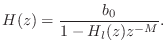
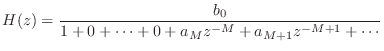
Equivalence of Parallel Combs to TDLs
It is easy to show that the TDL of Fig.2.19 is equivalent to a
parallel combination of three feedforward comb filters, each as in
Fig.2.23. To see this, we simply add the three comb-filter transfer
functions of Eq.![]() (2.3) and equate coefficients:
(2.3) and equate coefficients:
which implies
We see that parallel comb filters require more delay memory
(
![]() elements) than the corresponding TDL, which only
requires
elements) than the corresponding TDL, which only
requires
![]() elements.
elements.
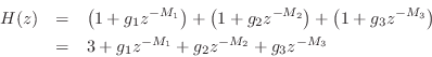
Equivalence of Series Combs to TDLs
It is also straightforward to show that a series combination of feedforward comb filters produces a sparsely tapped delay line as well. Considering the case of two sections, we have
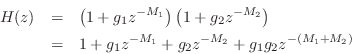
which yields
Time Varying Comb Filters
Comb filters can be changed slowly over time to produce the following digital audio ``effects'', among others:
Since all of these effects involve modulating delay length over time, and since time-varying delay lines typically require interpolation, these applications will be discussed after Chapter 5 which covers variable delay lines. For now, we will pursue what can be accomplished using fixed (time-invariant) delay lines. Perhaps the most important application is artificial reverberation, addressed in Chapter 3.
Next Section:
Feedback Delay Networks (FDN)
Previous Section:
Tapped Delay Line (TDL)


