


Digital Waveguide Models
In this chapter, we summarize the basic principles of digital waveguide models. Such models are used for efficient synthesis of string and wind musical instruments (and tonal percussion, etc.), as well as for artificial reverberation. They can be further used in modal synthesis by efficiently implementing a quasi harmonic series of modes in a single ``filtered delay loop''.
We begin with the simplest case of the infinitely long ideal vibrating string, and the model is unified with that of acoustic tubes. The resulting computational model turns out to be a simple bidirectional delay line. Next we consider what happens when a finite length of ideal string (or acoustic tube) is rigidly terminated on both ends, obtaining a delay-line loop. The delay-line loop provides a basic digital-waveguide synthesis model for (highly idealized) stringed and wind musical instruments. Next we study the simplest possible excitation for a digital waveguide string model, which is to move one of its (otherwise rigid) terminations. Excitation from ``initial conditions'' is then discussed, including the ideal plucked and struck string. Next we introduce damping into the digital waveguide, which is necessary to model realistic losses during vibration. This much modeling yields musically useful results. Another linear phenomenon we need to model, especially for piano strings, is dispersion, so that is taken up next. Following that, we consider general excitation of a string or tube model at any point along its length. Methods for calibrating models from recorded data are outlined, followed by modeling of coupled waveguides, and simple memoryless nonlinearities are introduced and analyzed.
Ideal Vibrating String
![\includegraphics[scale=0.9]{eps/FphysicalstringCopy}](http://www.dsprelated.com/josimages_new/pasp/img1307.png)
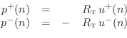
The ideal vibrating string is depicted in Fig.6.1. It is assumed to be perfectly flexible and elastic. Once ``plucked,'' it will vibrate forever in one plane as an energy conserving system. The mathematical theory of string vibration is considered in §B.6 and Appendix C. For present purposes, we only need some basic definitions and results.
Wave Equation
The wave equation for the ideal vibrating string may be written as
where we define the following notation:
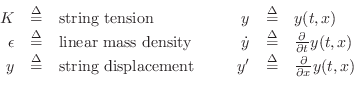 |
As discussed in Chapter 1, the wave equation in this form can be interpreted as a statement of Newton's second law,
Wave Equation Applications
The ideal-string wave equation applies to any perfectly elastic medium which is displaced along one dimension. For example, the air column of a clarinet or organ pipe can be modeled using the one-dimensional wave equation by substituting air-pressure deviation for string displacement, and longitudinal volume velocity for transverse string velocity. We refer to the general class of such media as one-dimensional waveguides. Extensions to two and three dimensions (and more, for the mathematically curious), are also possible (see §C.14) [518,520,55].
For a physical string model, at least three coupled waveguide models should be considered. Two correspond to transverse-wave vibrations in the horizontal and vertical planes (two polarizations of planar vibration); the third corresponds to longitudinal waves. For bowed strings, torsional waves should also be considered, since they affect bow-string dynamics [308,421]. In the piano, for key ranges in which the hammer strikes three strings simultaneously, nine coupled waveguides are required per key for a complete simulation (not including torsional waves); however, in a practical, high-quality, virtual piano, one waveguide per coupled string (modeling only the vertical, transverse plane) suffices quite well [42,43]. It is difficult to get by with fewer than the correct number of strings, however, because their detuning determines the entire amplitude envelope as well as beating and aftersound effects [543].
Traveling-Wave Solution
It can be readily checked (see §C.3 for details) that the lossless 1D wave equation

Note that we have
Sampled Traveling-Wave Solution
As discussed in more detail in Appendix C, the continuous traveling-wave
solution to the wave equation given in Eq.![]() (6.2) can be sampled
to yield
(6.2) can be sampled
to yield
where
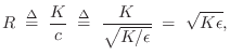
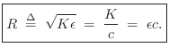
Wave Impedance
A concept of high practical utility is that of wave impedance, defined for vibrating strings as force divided by velocity. As derived in §C.7.2, the relevant force quantity in this case is minus the string tension times the string slope:
| (7.4) |
Physically, this can be regarded as the transverse force acting to the right on the string in the vertical direction. (Only transverse vibration is being considered.) In other words, the vertical component of a negative string slope pulls ``up'' on the segment of string to the right, and ``up'' is the positive direction for displacement, velocity, and now force. The traveling-wave decomposition of the force into force waves is thus given by (see §C.7.2 for a more detailed derivation)7.2

where we have defined the new notation
![]() for transverse velocity, and
for transverse velocity, and
The wave impedance simply relates force and velocity traveling waves:
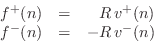
These relations may be called Ohm's law for traveling waves. Thus, in a traveling wave, force is always in phase with velocity (considering the minus sign in the left-going case to be associated with the direction of travel rather than a
The results of this section are derived in more detail in
Appendix C. However, all we need in practice for now are the
important Ohm's law relations for traveling-wave components given in
Eq.![]() (6.6).
(6.6).
Ideal Acoustic Tube
As discussed in §C.7.3, the most commonly used digital waveguide variables (``wave variables'') for acoustic tube simulation are traveling pressure and volume-velocity samples. These variables are exactly analogous to the traveling force and transverse-velocity waves used for vibrating string models.
The Ohm's law relations for acoustic-tube wave variables may be
written as follows (cf. Eq.![]() (6.6)):
(6.6)):
Here
| (7.8) |
where
In this formulation, the acoustic tube is assumed to contain only
traveling plane waves to the left and right. This is a
reasonable assumption for wavelengths ![]() much larger than the
tube diameter (
much larger than the
tube diameter (
![]() ). In this case, a change in the
tube cross-sectional area
). In this case, a change in the
tube cross-sectional area ![]() along the tube axis will cause lossless
scattering of incident plane waves. That is, the plane wave
splits into a transmitted and reflected component such that wave
energy is conserved (see Appendix C for a detailed derivation).
along the tube axis will cause lossless
scattering of incident plane waves. That is, the plane wave
splits into a transmitted and reflected component such that wave
energy is conserved (see Appendix C for a detailed derivation).
![\includegraphics[width=\twidth]{eps/KellyLochbaum}](http://www.dsprelated.com/josimages_new/pasp/img1343.png) |
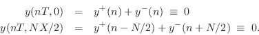
Figure 6.2 shows a piecewise cylindrical tube model of the
vocal tract and a corresponding digital simulation [245,297].
In the figure, ![]() denotes the reflection coefficient
associated with the first tube junction (where the cross-sectional
area changes), and
denotes the reflection coefficient
associated with the first tube junction (where the cross-sectional
area changes), and ![]() is the corresponding transmission
coefficient for traveling pressure plane waves. The
corresponding reflection and transmission coefficients for
volume velocity are
is the corresponding transmission
coefficient for traveling pressure plane waves. The
corresponding reflection and transmission coefficients for
volume velocity are ![]() and
and ![]() , respectively. Again,
see Appendix C for a complete derivation.
, respectively. Again,
see Appendix C for a complete derivation.
At higher frequencies, those for which
![]() , changes
in the tube cross-sectional area
, changes
in the tube cross-sectional area ![]() give rise to mode
conversion (which we will neglect in this chapter).
Mode conversion means that an incident plane wave (the simplest mode of
propagation in the tube) generally
scatters into waves traveling in many directions, not just the two
directions along the tube axis. Furthermore, even along the tube axis,
there are higher orders of mode propagation associated with ``node lines''
in the transverse plane (such as Bessel functions of integer order
[541]). When mode conversion occurs, it is necessary to keep
track of many components in a more general modal expansion of
the acoustic field [336,13,50]. We may say that
when a plane wave encounters a change in the cross-sectional tube
area, it is ``converted'' into a sum of propagation modes. The coefficients
(amplitude and phase) of the new modes are typically found by matching
boundary conditions. (Pressure and volume-velocity must be continuous
throughout the tube.)
give rise to mode
conversion (which we will neglect in this chapter).
Mode conversion means that an incident plane wave (the simplest mode of
propagation in the tube) generally
scatters into waves traveling in many directions, not just the two
directions along the tube axis. Furthermore, even along the tube axis,
there are higher orders of mode propagation associated with ``node lines''
in the transverse plane (such as Bessel functions of integer order
[541]). When mode conversion occurs, it is necessary to keep
track of many components in a more general modal expansion of
the acoustic field [336,13,50]. We may say that
when a plane wave encounters a change in the cross-sectional tube
area, it is ``converted'' into a sum of propagation modes. The coefficients
(amplitude and phase) of the new modes are typically found by matching
boundary conditions. (Pressure and volume-velocity must be continuous
throughout the tube.)
As mentioned above, in acoustic tubes we work with volume
velocity, because it is volume velocity that is conserved when a
wave propagates from one tube section to another. For plane waves in
open air, on the other hand, we use particle velocity, and in
this case, the wave impedance of open air is
![]() instead.
That is, the appropriate wave impedance in open air (not inside an
acoustic tube) is pressure divided by particle-velocity for any traveling
plane wave. If
instead.
That is, the appropriate wave impedance in open air (not inside an
acoustic tube) is pressure divided by particle-velocity for any traveling
plane wave. If ![]() denotes a sample of the volume-velocity
plane-wave traveling to the right in an acoustic tube of
cross-sectional area
denotes a sample of the volume-velocity
plane-wave traveling to the right in an acoustic tube of
cross-sectional area ![]() , and if
, and if ![]() denotes the corresponding
particle velocity, then we have
denotes the corresponding
particle velocity, then we have
Rigid Terminations
A rigid termination is the simplest case of a string (or tube)
termination. It imposes the constraint that the string (or air) cannot move
at the termination. (We'll look at the more practical case of a yielding
termination in §9.2.1.) If we terminate a length ![]() ideal string at
ideal string at
![]() and
and ![]() , we then have the ``boundary conditions''
, we then have the ``boundary conditions''
where ``
Applying the traveling-wave decomposition from Eq.![]() (6.2), we have
(6.2), we have
Therefore, solving for the reflected waves gives
| (7.10) | |||
| (7.11) |
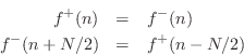
A digital simulation diagram for the rigidly terminated ideal string is shown in Fig.6.3. A ``virtual pickup'' is shown at the arbitrary location
![\includegraphics[width=\twidth]{eps/fterminatedstring}](http://www.dsprelated.com/josimages_new/pasp/img1360.png) |
Velocity Waves at a Rigid Termination
Since the displacement is always zero at a rigid termination, the velocity is also zero there:
Such inverting reflections for velocity waves at a rigid termination are identical for models of vibrating strings and acoustic tubes.
Force or Pressure Waves at a Rigid Termination
To find out how force or pressure waves recoil from a rigid
termination, we may convert velocity waves to force or velocity waves
by means of the Ohm's law relations of Eq.![]() (6.6) for strings
(or Eq.
(6.6) for strings
(or Eq.![]() (6.7) for acoustic tubes), and then use
Eq.
(6.7) for acoustic tubes), and then use
Eq.![]() (6.12), and then Eq.
(6.12), and then Eq.![]() (6.6) again:
(6.6) again:

Thus, force (and pressure) waves reflect from a rigid termination with no sign inversion:7.3
The reflections from a rigid termination in a digital-waveguide acoustic-tube simulation are exactly analogous:
Waveguide terminations in acoustic stringed and wind instruments are never perfectly rigid. However, they are typically passive, which means that waves at each frequency see a reflection coefficient not exceeding 1 in magnitude. Aspects of passive ``yielding'' terminations are discussed in §C.11.
Moving Rigid Termination
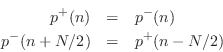
It is instructive to study the ``waveguide equivalent circuit'' of the simple case of a rigidly terminated ideal string with its left endpoint being moved by an external force, as shown in Fig.6.4. This case is relevant to bowed strings (§9.6) since, during time intervals in which the bow and string are stuck together, the bow provides a termination that divides the string into two largely isolated segments. The bow can therefore be regarded as a moving termination during ``sticking''.
![\includegraphics[width=\twidth]{eps/fMovingTermPhysical}](http://www.dsprelated.com/josimages_new/pasp/img1369.png)
Referring to Fig.6.4, the left termination of the
rigidly terminated ideal string is set in motion at time ![]() with a
constant velocity
with a
constant velocity ![]() . From Eq.
. From Eq.![]() (6.5), the wave impedance of
the ideal string is
(6.5), the wave impedance of
the ideal string is
![]() , where
, where ![]() is tension and
is tension and ![]() is mass density. Therefore, the upward force applied by the moving
termination is initially
is mass density. Therefore, the upward force applied by the moving
termination is initially ![]() . At time
. At time ![]() , the
traveling disturbance reaches a distance
, the
traveling disturbance reaches a distance ![]() from
from ![]() along the
string. Note that the string slope at the moving termination is given
by
along the
string. Note that the string slope at the moving termination is given
by
![]() , which derives
the fact that force waves are minus tension times slope waves.
(See §C.7.2 for a fuller discussion.)
, which derives
the fact that force waves are minus tension times slope waves.
(See §C.7.2 for a fuller discussion.)
Digital Waveguide Equivalent Circuits
![\includegraphics[width=\twidth]{eps/fMovingTerm}](http://www.dsprelated.com/josimages_new/pasp/img1374.png) |
Two digital waveguide ``equivalent circuits'' are shown in
Fig.6.5. In the velocity-wave case of Fig.6.5a,
the termination motion appears as an additive injection of a constant
velocity ![]() at the far left of the digital waveguide. At time 0,
this initiates a velocity step from 0 to
at the far left of the digital waveguide. At time 0,
this initiates a velocity step from 0 to ![]() traveling to the
right. When the traveling step-wave reaches the right termination, it
reflects with a sign inversion, thus sending back a ``canceling wave''
to the left. Behind the canceling wave, the velocity is zero, and the
string is not moving. When the canceling step-wave reaches the left
termination, it is inverted again and added to the externally injected
dc signal, thereby sending an amplitude
traveling to the
right. When the traveling step-wave reaches the right termination, it
reflects with a sign inversion, thus sending back a ``canceling wave''
to the left. Behind the canceling wave, the velocity is zero, and the
string is not moving. When the canceling step-wave reaches the left
termination, it is inverted again and added to the externally injected
dc signal, thereby sending an amplitude ![]() positive step-wave to
the right, overwriting the amplitude
positive step-wave to
the right, overwriting the amplitude ![]() signal in the upper rail.
This can be added to the amplitude
signal in the upper rail.
This can be added to the amplitude ![]() signal in the lower rail to
produce a net traveling velocity step of amplitude
signal in the lower rail to
produce a net traveling velocity step of amplitude ![]() traveling to
the right. This process repeats forever, resulting in traveling wave
components which grow without bound, but whose sum is always either
0 or
traveling to
the right. This process repeats forever, resulting in traveling wave
components which grow without bound, but whose sum is always either
0 or ![]() . Thus, at all times the string can be divided into two
segments, where the segment to the left is moving upward with speed
. Thus, at all times the string can be divided into two
segments, where the segment to the left is moving upward with speed
![]() , and the segment to the right is motionless.
, and the segment to the right is motionless.
At this point, it is a good exercise to try to mentally picture the
string shape during this process: Initially, since both the left end
support and the right-going velocity step are moving with constant
velocity ![]() , it is clear that the string shape is piece-wise linear, with
a negative-slope segment on the left adjoined to a zero-slope segment
on the right. When the velocity step reaches the right termination
and reflects to produce a canceling wave, everything to the left of
this wave remains a straight line which continues to move upward at
speed
, it is clear that the string shape is piece-wise linear, with
a negative-slope segment on the left adjoined to a zero-slope segment
on the right. When the velocity step reaches the right termination
and reflects to produce a canceling wave, everything to the left of
this wave remains a straight line which continues to move upward at
speed ![]() , while all points to the right of the canceling wave's
leading edge are not moving. What is the shape of this part of the
string? (The answer is given in the next paragraph, but try to
``see'' it first.)
, while all points to the right of the canceling wave's
leading edge are not moving. What is the shape of this part of the
string? (The answer is given in the next paragraph, but try to
``see'' it first.)
Animation of Moving String Termination and Digital Waveguide Models
In the force wave simulation of Fig.6.5b,7.4 the termination
motion appears as an additive injection of a constant force ![]() at the far left. At time 0, this initiates a force step from
0 to
at the far left. At time 0, this initiates a force step from
0 to ![]() traveling to the right. Since force waves are negated
slope waves multiplied by tension, i.e.,
traveling to the right. Since force waves are negated
slope waves multiplied by tension, i.e.,
![]() , the slope of
the string behind the traveling force step is
, the slope of
the string behind the traveling force step is ![]() . When the
traveling step-wave reaches the right termination, it reflects with
no sign inversion, thus sending back a doubling-wave to the left
which elevates the string force from
. When the
traveling step-wave reaches the right termination, it reflects with
no sign inversion, thus sending back a doubling-wave to the left
which elevates the string force from ![]() to
to ![]() . Behind this
wave, the slope is then
. Behind this
wave, the slope is then
![]() . This answers the question of
the previous paragraph: The string is in fact piecewise linear during
the first return reflection, consisting of two line segments with slope
. This answers the question of
the previous paragraph: The string is in fact piecewise linear during
the first return reflection, consisting of two line segments with slope
![]() on the left, and twice that on the right. When the return
step-wave reaches the left termination, it is reflected again and
added to the externally injected dc force signal, sending an amplitude
on the left, and twice that on the right. When the return
step-wave reaches the left termination, it is reflected again and
added to the externally injected dc force signal, sending an amplitude
![]() positive step-wave to the right (overwriting the amplitude
positive step-wave to the right (overwriting the amplitude
![]() signal in the upper rail). This can be added to the amplitude
signal in the upper rail). This can be added to the amplitude
![]() samples in the lower rail to produce a net traveling force step
in the string of amplitude
samples in the lower rail to produce a net traveling force step
in the string of amplitude ![]() traveling to the right. The slope
of the string behind this wave is
traveling to the right. The slope
of the string behind this wave is
![]() , and the slope in
front of this wave is still
, and the slope in
front of this wave is still ![]() . The force applied to the
string by the termination has risen to
. The force applied to the
string by the termination has risen to ![]() in order to keep the
velocity steady at
in order to keep the
velocity steady at ![]() . (We may interpret the
. (We may interpret the ![]() input as the
additional force needed each period to keep the termination moving
at speed
input as the
additional force needed each period to keep the termination moving
at speed ![]() --see the next paragraph below.)
This process repeats forever, resulting in
traveling wave components which grow without bound, and whose sum
(which is proportional to minus the physical string slope) also grows
without bound.7.5The string is always piecewise linear, consisting of
at most two linear segments having negative slopes which differ by
--see the next paragraph below.)
This process repeats forever, resulting in
traveling wave components which grow without bound, and whose sum
(which is proportional to minus the physical string slope) also grows
without bound.7.5The string is always piecewise linear, consisting of
at most two linear segments having negative slopes which differ by
![]() . A sequence of string displacement snapshots is shown in
Fig.6.6.
. A sequence of string displacement snapshots is shown in
Fig.6.6.
![\includegraphics[width=\twidth]{eps/moveterm}](http://www.dsprelated.com/josimages_new/pasp/img1386.png) |
Terminated String Impedance
Note that the impedance of the terminated string, seen from one
of its endpoints, is not the same thing as the wave impedance
![]() of the string itself. If the string is infinitely
long, they are the same. However, when there are reflections,
they must be included in the impedance calculation, giving it an
imaginary part. We may say that the impedance has a ``reactive''
component. The driving-point impedance of a rigidly terminated string
is ``purely reactive,'' and may be called a reactance (§7.1).
If
of the string itself. If the string is infinitely
long, they are the same. However, when there are reflections,
they must be included in the impedance calculation, giving it an
imaginary part. We may say that the impedance has a ``reactive''
component. The driving-point impedance of a rigidly terminated string
is ``purely reactive,'' and may be called a reactance (§7.1).
If ![]() denotes the force at the driving-point of the
string and
denotes the force at the driving-point of the
string and ![]() denotes its velocity, then the driving-point
impedance is given by (§7.1)
denotes its velocity, then the driving-point
impedance is given by (§7.1)
The Ideal Plucked String
The ideal plucked string is defined as an initial string
displacement and a zero initial velocity distribution [317]. More
generally, the initial displacement along the string ![]() and the
initial velocity distribution
and the
initial velocity distribution
![]() , for all
, for all ![]() , fully determine the
resulting motion in the absence of further excitation.
, fully determine the
resulting motion in the absence of further excitation.
An example of the appearance of the traveling-wave components and the resulting string shape shortly after plucking a doubly terminated string at a point one fourth along its length is shown in Fig.6.7. The negative traveling-wave portions can be thought of as inverted reflections of the incident waves, or as doubly flipped ``images'' which are coming from the other side of the terminations.
![\includegraphics[width=\twidth]{eps/f_t_waves_term}](http://www.dsprelated.com/josimages_new/pasp/img1393.png)
An example of an initial ``pluck'' excitation in a digital waveguide string model is shown in Fig.6.8. The circulating triangular components in Fig.6.8 are equivalent to the infinite train of initial images coming in from the left and right in Fig.6.7.
There is one fine-point to note for the discrete-time case:
We cannot admit a sharp corner
in the string since that would have infinite bandwidth which would alias
when sampled. Therefore, for the discrete-time case, we define the ideal
pluck to consist of an arbitrary shape as in
Fig.6.8 lowpass filtered to less than half
the sampling rate. Alternatively, we can simply require the initial
displacement shape to be bandlimited to spatial frequencies less than
![]() . Since all real strings have some degree of stiffness which
prevents the formation of perfectly sharp corners, and since real plectra
are never in contact with the string at only one point, and since the
frequencies we do allow span the full range of human hearing, the
bandlimited restriction is not limiting in any practical sense.
. Since all real strings have some degree of stiffness which
prevents the formation of perfectly sharp corners, and since real plectra
are never in contact with the string at only one point, and since the
frequencies we do allow span the full range of human hearing, the
bandlimited restriction is not limiting in any practical sense.
![\includegraphics[width=\twidth]{eps/fidealpluck}](http://www.dsprelated.com/josimages_new/pasp/img1395.png) |
Note that acceleration (or curvature) waves are a simple choice for
plucked string simulation, since the ideal pluck corresponds to an initial
impulse in the delay lines at the pluck point. Of course, since we
require a bandlimited excitation, the initial acceleration distribution
will be replaced by the impulse response of the anti-aliasing filter
chosen.
If the anti-aliasing filter chosen is the ideal lowpass filter cutting off
at ![]() , the initial acceleration
, the initial acceleration
![]() for the
ideal pluck becomes
for the
ideal pluck becomes
 sinc sinc |
(7.13) |
where
Aside from its obvious simplicity, there are two important benefits of obtaining an impulse-excited model: (1) an extremely efficient ``commuted synthesis'' algorithm can be readily defined (§8.7), and (2) linear prediction (and its relatives) can be readily used to calibrate the model to recordings of normally played tones on the modeled instrument. Linear Predictive Coding (LPC) has been used extensively in speech modeling [296,297,20]. LPC estimates the model filter coefficients under the assumption that the driving signal is spectrally flat. This assumption is valid when the input signal is (1) an impulse, or (2) white noise. In the basic LPC model for voiced speech, a periodic impulse train excites the model filter (which functions as the vocal tract), and for unvoiced speech, white noise is used as input.
In addition to plucked and struck strings, simplified bowed strings can be calibrated to recorded data as well using LPC [428,439]. In this simplified model, the bowed string is approximated as a periodically plucked string.
![\includegraphics[width=\twidth]{eps/fpluckaccel}](http://www.dsprelated.com/josimages_new/pasp/img1405.png) |
The Ideal Struck String
The ideal struck string [317] can be modeled by a zero
initial string displacement and a nonzero initial velocity
distribution. In concept, an inelastic ``hammer strike'' transfers an
``impulse'' of momentum to the string at time 0 along the striking
face of the hammer. (A more realistic model of a struck string will be
discussed in §9.3.1.)
An example of ``struck'' initial conditions is
shown in Fig.6.10 for a striking hammer having
a rectangular shape. Since
![]() ,7.6the initial velocity distribution can be integrated with respect to
,7.6the initial velocity distribution can be integrated with respect to ![]() from
from ![]() , divided by
, divided by ![]() , and negated in the upper rail to obtain
equivalent initial displacement waves [317]. Interestingly,
the initial displacement waves are not local (see also Appendix E).
, and negated in the upper rail to obtain
equivalent initial displacement waves [317]. Interestingly,
the initial displacement waves are not local (see also Appendix E).
![\includegraphics[width=\twidth]{eps/fidealstruck}](http://www.dsprelated.com/josimages_new/pasp/img1410.png)
The hammer strike itself may be considered to take zero time in the ideal case. A finite spatial width must be admitted for the hammer, however, even in the ideal case, because a zero width and a nonzero momentum transfer sends one (massless) point of the string immediately to infinity under infinite acceleration. In a discrete-time simulation, one sample represents an entire sampling interval, so a one-sample hammer width is well defined.
If the hammer velocity is ![]() , then the force against the
hammer due to pushing against the string wave impedance
is
, then the force against the
hammer due to pushing against the string wave impedance
is ![]() . The factor of
. The factor of ![]() arises because driving a point in
the string's interior is equivalent to driving two string endpoints in
``series,'' i.e., the reaction forces sum. If the hammer is itself a
dynamic system which has been ``thrown'' into the string,
as discussed in §9.3.1 below, the reaction
force slows the hammer over time, and the interaction is not impulsive, but
rather the momentum transfer takes place over a period of time.
arises because driving a point in
the string's interior is equivalent to driving two string endpoints in
``series,'' i.e., the reaction forces sum. If the hammer is itself a
dynamic system which has been ``thrown'' into the string,
as discussed in §9.3.1 below, the reaction
force slows the hammer over time, and the interaction is not impulsive, but
rather the momentum transfer takes place over a period of time.
The hammer-string collision is ideally inelastic since the string provides a reaction force that is equivalent to that of a dashpot. In the case of a pure mass striking a single point on the ideal string, the mass velocity decays exponentially, and an exponential wavefront emanates in both directions. In the musical acoustics literature for the piano, the hammer is often taken to be a nonlinear spring in series with a mass, as discuss further in §9.3.2. A commuted waveguide piano model including a linearized piano hammer is described in §9.4-§9.4.4. ``Wave digital hammer'' models, which employ a traveling-wave formulation of a lumped model and therefore analogous to a wave digital filter [136], are described in [523,56,42]. The ``wave digital'' modeling approach is introduced in §F.1.
The Damped Plucked String
Without damping, the ideal plucked string sounds more like a cheap electronic organ than a string because the sound is perfectly periodic and never decays. Static spectra are very boring to the ear. The discrete Fourier transform (DFT) of the initial ``string loop'' contents gives the Fourier series coefficients for the periodic tone produced.
The simplest change to the ideal wave equation of Eq.![]() (6.1) that
provides damping is to add a term proportional to velocity:
(6.1) that
provides damping is to add a term proportional to velocity:
Here,
Computational Savings
To illustrate how significant the computational savings can be,
consider the simulation of a ``damped guitar string'' model in
Fig.6.11. For simplicity, the length ![]() string is
rigidly terminated on both ends. Let the string be ``plucked'' by
initial conditions so that we need not couple an input mechanism to
the string. Also, let the output be simply the signal passing through
a particular delay element rather than the more realistic summation of
opposite elements in the bidirectional delay line. (A comb filter
corresponding to pluck position can be added in series later.)
string is
rigidly terminated on both ends. Let the string be ``plucked'' by
initial conditions so that we need not couple an input mechanism to
the string. Also, let the output be simply the signal passing through
a particular delay element rather than the more realistic summation of
opposite elements in the bidirectional delay line. (A comb filter
corresponding to pluck position can be added in series later.)
![\includegraphics[width=\twidth]{eps/fstring}](http://www.dsprelated.com/josimages_new/pasp/img1418.png) |
In this string simulator, there is a loop of delay containing
![]() samples where
samples where ![]() is the desired pitch of the string. Because
there is no input/output coupling, we may lump all of the losses at
a single point in the delay loop. Furthermore, the two reflecting
terminations (gain factors of
is the desired pitch of the string. Because
there is no input/output coupling, we may lump all of the losses at
a single point in the delay loop. Furthermore, the two reflecting
terminations (gain factors of ![]() ) may be commuted so as to cancel them.
Finally, the right-going delay may be combined with the left-going delay to
give a single, length
) may be commuted so as to cancel them.
Finally, the right-going delay may be combined with the left-going delay to
give a single, length ![]() , delay line. The result of these inaudible
simplifications is shown in Fig. 6.12.
, delay line. The result of these inaudible
simplifications is shown in Fig. 6.12.
![\includegraphics[width=\twidth]{eps/fsstring}](http://www.dsprelated.com/josimages_new/pasp/img1421.png) |
If the sampling rate is ![]() kHz and the desired pitch is
kHz and the desired pitch is ![]() Hz, the loop delay equals
Hz, the loop delay equals ![]() samples. Since delay lines are
efficiently implemented as circular buffers, the cost of implementation is
normally dominated by the loss factors, each one requiring a multiply
every sample, in general. (Losses of the form
samples. Since delay lines are
efficiently implemented as circular buffers, the cost of implementation is
normally dominated by the loss factors, each one requiring a multiply
every sample, in general. (Losses of the form ![]() ,
,
![]() , etc., can be efficiently implemented using shifts and
adds.) Thus, the consolidation of loss factors has reduced computational
complexity by three orders of magnitude, i.e., by a factor of
, etc., can be efficiently implemented using shifts and
adds.) Thus, the consolidation of loss factors has reduced computational
complexity by three orders of magnitude, i.e., by a factor of
![]() in this case. However, the physical accuracy of the simulation has
not been compromised. In fact, the accuracy is improved because
the
in this case. However, the physical accuracy of the simulation has
not been compromised. In fact, the accuracy is improved because
the ![]() round-off errors per period arising from repeated multiplication
by
round-off errors per period arising from repeated multiplication
by ![]() have been replaced by a single round-off error per period
in the multiplication by
have been replaced by a single round-off error per period
in the multiplication by ![]() .
.
Frequency-Dependent Damping
In real vibrating strings, damping typically increases with frequency
for a variety of physical reasons
[73,77]. A simple
modification [392] to Eq.![]() (6.14) yielding
frequency-dependent damping is
(6.14) yielding
frequency-dependent damping is
The result of adding such damping terms to the wave equation is that
traveling waves on the string decay at frequency-dependent
rates. This means the loss factors ![]() of the previous section
should really be digital filters having gains which decrease
with frequency (and never exceed
of the previous section
should really be digital filters having gains which decrease
with frequency (and never exceed ![]() for stability of the loop).
These filters commute with delay elements because they are
linear and time invariant (LTI) [449]. Thus,
following the reasoning of the previous section, they can be lumped at
a single point in the digital waveguide. Let
for stability of the loop).
These filters commute with delay elements because they are
linear and time invariant (LTI) [449]. Thus,
following the reasoning of the previous section, they can be lumped at
a single point in the digital waveguide. Let
![]() denote the
resulting string loop filter (replacing
denote the
resulting string loop filter (replacing ![]() in
Fig.6.127.7). We have the stability (passivity)
constraint
in
Fig.6.127.7). We have the stability (passivity)
constraint
![]() , and making the filter
linear phase (constant delay at all frequencies) will restrict
consideration to symmetric FIR filters only.
, and making the filter
linear phase (constant delay at all frequencies) will restrict
consideration to symmetric FIR filters only.
Restriction to FIR filters yields the important advantage of keeping the approximation problem convex in the weighted least-squares norm. Convexity of a norm means that gradient-based search techniques can be used to find a global miminizer of the error norm without exhaustive search [64],[428, Appendix A].
The linear-phase requirement halves the degrees of freedom in the filter
coefficients. That is, given
![]() for
for ![]() , the coefficients
, the coefficients
![]() are also determined. The loss-filter frequency response
can be written in terms of its (impulse response) coefficients as
are also determined. The loss-filter frequency response
can be written in terms of its (impulse response) coefficients as
A further degree of freedom is eliminated from the loss-filter
approximation by assuming all losses are insignificant at 0 Hz so that
![]() (taking the approximation error to be zero at
(taking the approximation error to be zero at
![]() ). This means the coefficients of the FIR filter must sum to
). This means the coefficients of the FIR filter must sum to ![]() .
If the length of the filter is
.
If the length of the filter is
![]() , we have
, we have
The Stiff String
Stiffness in a vibrating string introduces a restoring force proportional to the bending angle of the string. As discussed further in §C.6, the usual stiffness term added to the wave equation for the ideal string yields
Stiff-string models are commonly used in piano synthesis. In §9.4, further details of string models used in piano synthesis are described (§9.4.1).
Experiments with modified recordings of acoustic classical guitars indicate that overtone inharmonicity due to string-stiffness is generally not audible in nylon-string guitars, although just-noticeable-differences are possible for the 6th (lowest) string [225]. Such experiments may be carried out by retuning the partial overtones in a recorded sound sample so that they become exact harmonics. Such retuning is straightforward using sinusoidal modeling techniques [359,456].
Stiff String Synthesis Models
![\includegraphics[width=\twidth]{eps/flstifftstring}](http://www.dsprelated.com/josimages_new/pasp/img1441.png)
An ideal stiff-string synthesis model is drawn in
Fig. 6.13 [10]. See
§C.6 for a detailed derivation. The delay-line length
![]() is the number of samples in
is the number of samples in ![]() periods at frequency
periods at frequency ![]() , where
, where
![]() is the number of the highest partial supported (normally the last
one before
is the number of the highest partial supported (normally the last
one before ![]() ). This is the counterpart of
Fig. 6.12 which depicted ideal-string damping which
was lumped at a single point in the delay-line loop. For the
ideal stiff string, however, (no damping), it is dispersion
filtering that is lumped at a single point of the loop. Dispersion
can be lumped like damping because it, too, is a linear,
time-invariant (LTI) filtering of a propagating wave. Because it is
LTI, dispersion-filtering commutes with other LTI systems in
series, such as delay elements. The allpass filter in
Fig.C.9 corresponds to filter
). This is the counterpart of
Fig. 6.12 which depicted ideal-string damping which
was lumped at a single point in the delay-line loop. For the
ideal stiff string, however, (no damping), it is dispersion
filtering that is lumped at a single point of the loop. Dispersion
can be lumped like damping because it, too, is a linear,
time-invariant (LTI) filtering of a propagating wave. Because it is
LTI, dispersion-filtering commutes with other LTI systems in
series, such as delay elements. The allpass filter in
Fig.C.9 corresponds to filter ![]() in Fig.9.2 for
the Extended Karplus-Strong algorithm. In practice, losses are also
included for realistic string behavior (filter
in Fig.9.2 for
the Extended Karplus-Strong algorithm. In practice, losses are also
included for realistic string behavior (filter ![]() in
Fig.9.2).
in
Fig.9.2).
Allpass filters were introduced in §2.8, and a fairly comprehensive summary is given in Book II of this series [449, Appendix C].7.8The general transfer function for an allpass filter is given (in the real, single-input, single-output case) by
Section 6.11 below discusses some
methods for designing stiffness allpass filters ![]() from
measurements of stiff vibrating strings, and
§9.4.1 gives further details for the case of piano
string modeling.
from
measurements of stiff vibrating strings, and
§9.4.1 gives further details for the case of piano
string modeling.
The Externally Excited String
Sections 6.5 and 6.6 illustrated plucking or striking the string by means of initial conditions: an initial displacement for plucking and an initial velocity distribution for striking. Such a description parallels that found in many textbooks on acoustics, such as [317]. However, if the string is already in motion, as it often is in normal usage, it is more natural to excite the string externally by the equivalent of a ``pick'' or ``hammer'' as is done in the real world instrument.
Figure 6.14 depicts a rigidly terminated string with an
external excitation input. The wave variable ![]() can be set to
acceleration, velocity, or displacement, as appropriate. (Choosing
force waves would require eliminating the sign inversions at the
terminations.) The external input is denoted
can be set to
acceleration, velocity, or displacement, as appropriate. (Choosing
force waves would require eliminating the sign inversions at the
terminations.) The external input is denoted
![]() to indicate
that it is an additive incremental input, superimposing with the
existing string state.
to indicate
that it is an additive incremental input, superimposing with the
existing string state.
![\includegraphics[width=\twidth]{eps/fpluckedstring}](http://www.dsprelated.com/josimages_new/pasp/img1453.png)
For idealized plucked strings, we may take ![]() (acceleration), and
(acceleration), and
![]() can be a single nonzero sample, or impulse, at the plucking instant. As
always, bandlimited interpolation can be used to provide a non-integer time
or position. In the latter case, there would be two or more summers along
both the upper and lower rails, separated by unit delays. More generally,
the string may be plucked by a force distribution
can be a single nonzero sample, or impulse, at the plucking instant. As
always, bandlimited interpolation can be used to provide a non-integer time
or position. In the latter case, there would be two or more summers along
both the upper and lower rails, separated by unit delays. More generally,
the string may be plucked by a force distribution
![]() .
The applied force at a point can be translated to the corresponding
velocity increment via the wave impedance
.
The applied force at a point can be translated to the corresponding
velocity increment via the wave impedance ![]() :
:
 |
(7.15) |
where
Note that the force applied by a rigid, stationary pick or hammer varies with the state of a vibrating string. Also, when a pick or hammer makes contact with the string, it partially terminates the string, resulting in reflected waves in each direction. A simple model for the termination would be a mass affixed to the string at the excitation point. (This model is pursued in §9.3.1.) A more general model would be an arbitrary impedance and force source affixed to the string at the excitation point during the excitation event. This is a special case of the ``loaded waveguide junction,'' discussed in §C.12. In the waveguide model for bowed strings (§9.6), the bow-string interface is modeled as a nonlinear scattering junction.
Equivalent Forms
In a physical piano string, as a specific example, the hammer strikes the string between its two inputs, some distance from the agraffe and far from the bridge. This corresponds to the diagram in Fig.6.15, where the delay lines are again arranged for clarity of physical interpretation. Figure 6.15 is almost identical to Fig.6.14, except that the delay lines now contain samples of traveling force waves, and the bridge is allowed to vibrate, resulting in a filtered reflection at the bridge (see §9.2.1 for a derivation of the bridge filter). The hammer-string interaction force-pulse is summed into both the left- and right-going delay lines, corresponding to sending the same pulse toward both ends of the string from the hammer. Force waves are discussed further in §C.7.2.
![\includegraphics[width=\twidth]{eps/pianoInteriorStringExcitation}](http://www.dsprelated.com/josimages_new/pasp/img1457.png)
![\includegraphics[width=\twidth]{eps/pianoSimplifiedInteriorStringExcitation}](http://www.dsprelated.com/josimages_new/pasp/img1458.png)
By commutativity of linear, time-invariant elements, Figure 6.15 can be immediately simplified to the form shown in Fig.6.16, in which each delay line corresponds to the travel time in both directions on each string segment. From a structural point of view, we have a conventional filtered delay loop plus a second input which sums into the loop somewhere inside the delay line. The output is shown coming from the middle of the larger delay line, which gives physically correct timing, but in practice, the output can be taken from anywhere in the feedback loop. It is probably preferable in practice to take the output from the loop-delay-line input. That way, other response latencies in the overall system can be compensated.
![\includegraphics[width=\twidth]{eps/pianoSimplifiedISEExtracted}](http://www.dsprelated.com/josimages_new/pasp/img1459.png) |
An alternate structure equivalent to Fig.6.16 is shown in Fig.6.17, in which the second input injection is factored out into a separate comb-filtering of the input. The comb-filter delay equals the delay between the two inputs in Fig.6.16, and the delay in the feedback loop equals the sum of both delays in Fig.6.16. In this case, the string is modeled using a simple filtered delay loop, and the striking-force signal is separately filtered by a comb filter corresponding to the striking-point along the string.
Algebraic derivation
The above equivalent forms are readily verified by deriving the
transfer function from the striking-force input ![]() to the output
force signal
to the output
force signal ![]()
Referring to Fig.6.15, denote the input
hammer-strike ![]() transform by
transform by ![]() and the output signal
and the output signal ![]() transform by
transform by ![]() . Also denote the loop-filter transfer function
by
. Also denote the loop-filter transfer function
by ![]() . By inspection of the figure, we can write
. By inspection of the figure, we can write
The final factored form above corresponds to the final equivalent form shown in Fig.6.17.
Related Forms
We see from the preceding example that a filtered-delay loop (a
feedback comb-filter using filtered feedback, with delay-line length
![]() in the above example) simulates a vibrating string in a manner
that is independent of where the excitation is applied. To
simulate the effect of a particular excitation point, a feedforward
comb-filter may be placed in series with the filtered delay loop.
Such a ``pluck position'' illusion may be applied to any basic string
synthesis algorithm, such as the EKS [428,207].
in the above example) simulates a vibrating string in a manner
that is independent of where the excitation is applied. To
simulate the effect of a particular excitation point, a feedforward
comb-filter may be placed in series with the filtered delay loop.
Such a ``pluck position'' illusion may be applied to any basic string
synthesis algorithm, such as the EKS [428,207].
By an exactly analogous derivation, a single feedforward comb filter can be used to simulate the location of a linearized magnetic pickup [200] on a simulated electric guitar string. An ideal pickup is formally the transpose of an excitation. For a discussion of filter transposition (using Mason's gain theorem [301,302]), see, e.g., [333,449].7.9
The comb filtering can of course also be implemented after the filtered delay loop, again by commutativity. This may be desirable in situations in which comb filtering is one of many options provided for in the ``effects section'' of a synthesizer. Post-processing comb filters are often used in reverberator design and in virtual pickup simulation.
![\includegraphics[width=\twidth]{eps/pianoSecondStringTap}](http://www.dsprelated.com/josimages_new/pasp/img1467.png) |
The comb-filtering can also be conveniently implemented using a second
tap from the appropriate delay element in the filtered delay loop
simulation of the string, as depicted in
Fig.6.18. The new tap output is simply
summed (or differenced, depending on loop implementation) with the
filtered delay loop output. Note that making the new tap a moving,
interpolating tap (e.g., using linear interpolation), a flanging
effect is available. The tap-gain ![]() can be brought out as a
musically useful timbre control that goes beyond precise physical
simulation (e.g., it can be made negative). Adding more moving taps
and summing/differencing their outputs, with optional scale factors,
provides an economical chorus or Leslie effect. These
extra delay effects cost no extra memory since they utilize the memory
that's already needed for the string simulation. While such effects
are not traditionally applied to piano sounds, they are applied to
electric piano sounds which can also be simulated using the same basic
technique.
can be brought out as a
musically useful timbre control that goes beyond precise physical
simulation (e.g., it can be made negative). Adding more moving taps
and summing/differencing their outputs, with optional scale factors,
provides an economical chorus or Leslie effect. These
extra delay effects cost no extra memory since they utilize the memory
that's already needed for the string simulation. While such effects
are not traditionally applied to piano sounds, they are applied to
electric piano sounds which can also be simulated using the same basic
technique.
Summary
In summary, two feedforward comb filters and one feedback comb filter arranged in series (in any order) can be interpreted as a physical model of a vibrating string driven at one point along the string and observed at a different point along the string. The two feedforward comb-filter delays correspond to the excitation and pickup locations along the string, while the amount of feedback-loop delay controls the fundamental frequency of vibration. A filter in the feedback loop determines the decay rate and fine tuning of the partial overtones.
Loop Filter Identification
In §6.7 we discussed damping filters for vibrating string models, and in §6.9 we discussed dispersion filters. For vibrating strings which are well described by a linear, time-invariant (LTI) partial differential equation, damping and dispersion filtering are the only deviations possible from the ideal string string discussed in §6.1.
The ideal damping filter is ``zero phase'' (or linear phase) [449],7.10while the ideal dispersion filter is ``allpass'' (as described in §6.9.1). Since every desired frequency response can be decomposed into a zero-phase frequency-response in series with an allpass frequency-response, we may design a single loop filter whose amplitude response gives the desired damping as a function of frequency, and whose phase response gives the desired dispersion vs. frequency. The next subsection summarizes some methods based on this approach. The following two subsections discuss methods for the design of damping and dispersion filters separately.
General Loop-Filter Design
For general loop-filter design in vibrating string models (as well as in woodwind and brass instrument bore models), we wish to minimize [428, pp. 182-184]:
- Errors in partial overtone decay times
- Errors in partial overtone tuning
There are numerous methods for designing the string loop filter
![]() based on measurements of real string behavior. In
[428], a variety of methods for system identification
[288] were explored for this purpose, including
``periodic linear prediction'' in which a linear combination of a
small group of samples is used to predict a sample one period away
from the midpoint of the group. An approach based on a genetic
algorithm is described in [378]; in that work,
the error measure used with the genetic algorithm is based on
properties of human perception of short-time spectra, as is now
standard practice in digital audio coding [62].
Overviews of other approaches appear in [29] and
[508].
based on measurements of real string behavior. In
[428], a variety of methods for system identification
[288] were explored for this purpose, including
``periodic linear prediction'' in which a linear combination of a
small group of samples is used to predict a sample one period away
from the midpoint of the group. An approach based on a genetic
algorithm is described in [378]; in that work,
the error measure used with the genetic algorithm is based on
properties of human perception of short-time spectra, as is now
standard practice in digital audio coding [62].
Overviews of other approaches appear in [29] and
[508].
Below is an outline of a simple and effective method used (ca. 1995) to design loop filters for some of the Sondius sound examples:
- Estimate the fundamental frequency (see §6.11.4 below)
- Set a Hamming FFT-window length to approximately four periods
- Compute the short-time Fourier transform (STFT)
- Perform a sinusoidal modeling analysis [466] to
- -
- detect peaks in each spectral frame, and
- -
- connect peaks through time to form amplitude envelopes
- Fit an exponential to each amplitude envelope
- Prepare the desired frequency-response, sampled at the harmonic
frequencies of the delay-line loop without the loop filter. At
each harmonic frequency,
- -
- the nearest-partial decay-rate gives the desired loop-filter gains,
- -
- the nearest-partial peak-frequency give the desired loop-filter phase delay.
- Use a phase-sensitive filter-design method such as invfreqz in matlab to design the desired loop filter from its frequency-response samples (further details below).
Physically, amplitude envelopes are expected to decay exponentially, although coupling phenomena may obscure the overall exponential trend. On a dB scale, exponential decay is a straight line. Therefore, a simple method of estimating the exponential decay time-constant for each overtone frequency is to fit a straight line to its amplitude envelope and use the slope of the fitted line to compute the decay time-constant. For example, the matlab function polyfit can be used for this purpose (where the requested polynomial order is set to 1). Since ``beating'' is typical in the amplitude envelopes, a refinement is to replace the raw amplitude envelope by a piecewise linear envelope that connects the upper local maxima in the raw amplitude envelope. The estimated decay-rate for each overtone determines a sample of the loop-filter amplitude response at the overtone frequency. Similarly, the overtone frequency determines a sample of the loop-filter phase response.
Taken together, the measured overtone decay rates and tunings determine samples of the complex frequency response of the desired loop filter. The matlab function invfreqz7.11 can be used to convert these complex samples into recursive filter coefficients (see §8.6.4 for a related example). A weighting function inversely proportional to frequency is recommended. Additionally, Steiglitz-McBride iterations can improve the results [287], [428, pp. 101-103]. Matlab's version of invfreqz has an iteration-count argument for specifying the number of Steiglitz-McBride iterations. The maximum filter-gain versus frequency should be computed, and the filter should be renormalized, if necessary, to ensure that its gain does not exceed 1 at any frequency; one good setting is that which matches the overall decay rate of the original recording.
Damping Filter Design
When dispersion can be neglected (as it typically can in many cases, such as for guitar strings), we may use linear-phase filter design methods, such as provided by the functions remez, firls, and fir2 in matlab. Since strings are usually very lightly damped, such linear-phase filter designs give high quality at very low orders. Another approach is to fit a low-order IIR filter, such as by applying invfreqz to a minimum-phase version of the desired amplitude response, and then subtract the phase-response of the resulting filter from the desired phase-response used in a subsequent allpass design. (Alternatively, the phase response of the loop filter can simply be neglected, as long as tuning is unaffected. If tuning is affected, the tuning allpass can be adjusted to compensate.)
Dispersion Filter Design
A pure dispersion filter is an ideal allpass filter. That is, it has a gain of 1 at all frequencies and only delays a signal in a frequency-dependent manner. The need for such filtering in piano string models is discussed in §9.4.1.
There is a good amount of literature on the topic of allpass filter design. Generally, they fall into the categories of optimized parametric, closed-form parametric, and nonparametric methods. Optimized parametric methods can produce allpass filters with optimal group-delay characteristics in some sense [272,271]. Closed-form parametric methods provide coefficient formulas as a function of a desired parameter such as ``inharmonicity'' [368]. Nonparametric methods are generally based on measured signals and/or spectra, and while they are suboptimal, they can be used to design very large-order allpass filters, and the errors can usually be made arbitrarily small by increasing the order [551,369,42,41,1], [428, pp. 60,172]. In music applications, it is usually the case that the ``optimality'' criterion is unknown because it depends on aspects of sound perception (see, for example, [211,384]). As a result, perceptually weighted nonparametric methods can often outperform optimal parametric methods in terms of cost/performance [2].
In historical order, some of the allpass filter-design methods are as
follows: A modification of the method in [551] was
suggested for designing allpass filters having a phase delay
corresponding to the delay profile needed for a stiff string
simulation [428, pp. 60,172]. The method of
[551] was streamlined in [369]. In
[77], piano strings were modeled using
finite-difference techniques. An update on this approach appears in
[45]. In [340], high quality stiff-string
sounds were demonstrated using high-order allpass filters in a digital
waveguide model. In [384], this work was extended by
applying a least-squares allpass-design method [272]
and a spectral Bark-warping technique [459] to the
problem of calibrating an allpass filter of arbitrary order to
recorded piano strings. They were able to correctly tune the first
several tens of partials for any natural piano string with a total
allpass order of 20 or less. Additionally, minimization of the
![]() norm [271] has been used to calibrate a series of
allpass-filter sections [42,41], and a dynamically
tunable method, based on Thiran's closed-form, maximally flat
group-delay allpass filter design formulas (§4.3), was
proposed in [368]. An improved closed-form
solution appears in [1] based on an elementary
method for the robust design of very high-order allpass filters.
norm [271] has been used to calibrate a series of
allpass-filter sections [42,41], and a dynamically
tunable method, based on Thiran's closed-form, maximally flat
group-delay allpass filter design formulas (§4.3), was
proposed in [368]. An improved closed-form
solution appears in [1] based on an elementary
method for the robust design of very high-order allpass filters.
Fundamental Frequency Estimation
As mentioned in §6.11.2 above, it is advisable to estimate the fundamental frequency of vibration (often called ``F0'') in order that the partial overtones are well resolved while maintaining maximum time resolution for estimating the decay time-constant.
Below is a summary of the F0 estimation method used in calibrating loop filters with good results [471]:
- Take an FFT of the middle third of a recorded plucked string tone.
- Find the frequencies and amplitudes of the largest
 peaks, where
is chosen so that the retained peaks all have a reasonable
signal-to-noise ratio.
peaks, where
is chosen so that the retained peaks all have a reasonable
signal-to-noise ratio.
- Form a histogram of peak spacing

- The pitch estimate
 is defined as the most common spacing
in the histogram.
is defined as the most common spacing
in the histogram.
Approximate Maximum Likelihood F0 Estimation
In applications for which the fundamental frequency F0 must be
measured very accurately in a periodic signal,
the estimate
![]() obtained by the above
algorithm can be refined using a gradient search which matches a
so-called ``harmonic comb'' to the magnitude spectrum of an
interpolated FFT
obtained by the above
algorithm can be refined using a gradient search which matches a
so-called ``harmonic comb'' to the magnitude spectrum of an
interpolated FFT ![]() :
:
![$\displaystyle {\hat f}_0 \isdefs \arg\max_{{\hat f}_0} \sum_{k=1}^K \log\left[\...
...f}_0} \prod_{k=1}^K \left[\left\vert X(k{\hat f}_0)\right\vert+\epsilon\right]
$](http://www.dsprelated.com/josimages_new/pasp/img1471.png)
Note that freely vibrating strings are not exactly periodic due to
exponenential decay, coupling effects, and stiffness (which stretches
harmonics into quasiharmonic overtones, as explained
in §6.9). However, non-stiff strings can often be
analyzed as having approximately harmonic spectra (
![]() periodic time waveform) over a limited time frame.
periodic time waveform) over a limited time frame.
Since string spectra typically exhibit harmonically spaced
nulls associated
with the excitation and/or observation points, as well as from other
phenomena such as recording multipath and/or reverberation, it is
advisable to restrict ![]() to a range that does not include any
spectral nulls (or simply omit index
to a range that does not include any
spectral nulls (or simply omit index ![]() when
when
![]() is
too close to a spectral null),
since even one spectral null can push the product of
peak amplitudes to a very small value. As a practical matter, it is
important to inspect the magnitude spectra of the data manually to
ensure that a robust row of peaks is being matched by the harmonic
comb. For example, a display of the frame magnitude spectrum overlaid
with vertical lines at the optimized harmonic-comb frequencies yields
an effective picture of the F0 estimate in which typical problems
(such as octave errors) are readily seen.
is
too close to a spectral null),
since even one spectral null can push the product of
peak amplitudes to a very small value. As a practical matter, it is
important to inspect the magnitude spectra of the data manually to
ensure that a robust row of peaks is being matched by the harmonic
comb. For example, a display of the frame magnitude spectrum overlaid
with vertical lines at the optimized harmonic-comb frequencies yields
an effective picture of the F0 estimate in which typical problems
(such as octave errors) are readily seen.
References on F0 Estimation
An often-cited book on classical methods for pitch detection, particularly for voice, is that by Hess [192]. The harmonic comb method can be considered an approximate maximum-likelihood pitch estimator, and more accurate maximum-likelihood methods have been worked out [114,547,376,377]. More recently, Klapuri has been developing some promising methods for multiple pitch estimation [254,253,252].7.12A comparison of real-time pitch-tracking algorithms applied to guitar is given in [260], with consideration of latency (time delay).
Extension to Stiff Strings
An advantage of the harmonic-comb method, as well as other frequency-domain maximum-likelihood pitch-estimation methods, is that it is easily extended to accommodate stiff strings. For this, the stretch-factor in the spectral-peak center-frequencies can be estimated--the so-called coefficient of inharmonicity, and then the harmonic-comb (or other maximum-likelihood spectral-matching template) can be stretched by the same amount, so that when set to the correct pitch, the template matches the data spectrum more accurately than if harmonicity is assumed.
EDR-Based Loop-Filter Design
This section discusses use of the Energy Decay Relief (EDR) (§3.2.2) to measure the decay times of the partial overtones in a recorded vibrating string.
First we derive what to expect in the case of a simplified string
model along the lines discussed in §6.7 above. Assume we
have the synthesis model of Fig.6.12, where now the loss
factor ![]() is replaced by the digital filter
is replaced by the digital filter ![]() that we wish
to design. Let
that we wish
to design. Let
![]() denote the contents of the delay line as a
vector at time
denote the contents of the delay line as a
vector at time ![]() , with
, with
![]() denoting the initial contents of the
delay line.
denoting the initial contents of the
delay line.
For simplicity, we define the EDR based on a length ![]() DFT of the delay-line
vector
DFT of the delay-line
vector
![]() , and use a rectangular window with a ``hop size'' of
, and use a rectangular window with a ``hop size'' of ![]() samples,
i.e.,
samples,
i.e.,
Applying the definition of the EDR (§3.2.2) to this short-time spectrum gives
We therefore have the following recursion for successive EDR time-slices:7.13
This analysis can be generalized to a time-varying model in which the
loop filter ![]() is allowed to change once per ``period''
is allowed to change once per ``period''
![]() .7.14
.7.14
An online laboratory exercise covering the practical details of measuring overtone decay-times and designing a corresponding loop filter is given in [280].
String Coupling Effects
It turns out that a single digital waveguide provides a relatively static-sounding string synthesizer. This is because several coupling mechanisms exist in natural string instruments. The overtones in coupled strings exhibit more interesting amplitude envelopes over time. Coupling between different strings is not the only important coupling phenomenon. In a real string, there are two orthogonal planes of transverse vibration which are intrinsically coupled to each other [181]. There is also intrinsic coupling between transverse vibrational waves and longitudinal waves (see §B.6).
Horizontal and Vertical Transverse Waves
The transverse waves considered up to now represent string vibration
only in a single two-dimensional plane. One such plane can be chosen
as being perpendicular to the top plate of a stringed musical instrument. We
will call this the ![]() plane and refer to it as the vertical
plane of polarization for transverse waves on a string (or simply the
vertical component of the transverse vibration). To more fully
model a real vibrating string, we also need to include transverse waves
in the
plane and refer to it as the vertical
plane of polarization for transverse waves on a string (or simply the
vertical component of the transverse vibration). To more fully
model a real vibrating string, we also need to include transverse waves
in the ![]() plane, i.e., a horizontal plane of polarization (or
horizontal component of vibration). Any polarization for transverse
traveling waves can be represented as a linear combination of
horizontal and vertical polarizations, and general transverse string
vibration in 3D can be expressed as a linear superposition of
vibration in any two distinct polarizations.
plane, i.e., a horizontal plane of polarization (or
horizontal component of vibration). Any polarization for transverse
traveling waves can be represented as a linear combination of
horizontal and vertical polarizations, and general transverse string
vibration in 3D can be expressed as a linear superposition of
vibration in any two distinct polarizations.
 |
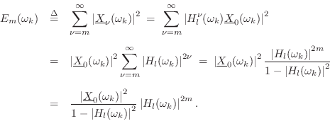
If string terminations were perfectly rigid, the horizontal polarization would be largely independent of the vertical polarization, and an accurate model would consist of two identical, uncoupled, filtered delay loops (FDL), as depicted in Fig.6.19. One FDL models vertical force waves while the other models horizontal force waves. This model neglects the small degree of nonlinear coupling between horizontal and vertical traveling waves along the length of the string--valid when the string slope is much less than unity (see §B.6).
Note that the model for two orthogonal planes of vibration on a single string is identical to that for a single plane of vibration on two different strings.
Coupled Horizontal and Vertical Waves
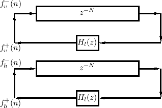
No vibrating string in musical acoustics is truly rigidly terminated, because such a string would produce no sound through the body of the instrument.7.15Yielding terminations result in coupling of the horizontal and vertical planes of vibration. In typical acoustic stringed instruments, nearly all of this coupling takes place at the bridge of the instrument.
 |
Figure 6.20 illustrates the more realistic case of
two planes of vibration which are linearly coupled at one end
of the string (the ``bridge''). Denoting the traveling force waves
entering the bridge from the vertical and horizontal vibration
components by ![]() and
and ![]() , respectively, the outgoing
waves in each plane are given by
, respectively, the outgoing
waves in each plane are given by
![$\displaystyle \left[\begin{array}{c} F_v^-(z) \\ [2pt] F_h^-(z) \end{array}\rig...
...] \left[\begin{array}{c} F_v^+(z) \\ [2pt] F_h^+(z) \end{array}\right] \protect$](http://www.dsprelated.com/josimages_new/pasp/img1494.png)
as shown in the figure.
In physically symmetric situations, we expect
![]() .
That is, the transfer function from horizontal to vertical waves is
normally the same as the transfer function from vertical to horizontal
waves.
.
That is, the transfer function from horizontal to vertical waves is
normally the same as the transfer function from vertical to horizontal
waves.
If we consider a single frequency ![]() , then the coupling matrix
with
, then the coupling matrix
with
![]() is a constant (generally complex) matrix (where
is a constant (generally complex) matrix (where
![]() denotes the sampling interval as usual). An eigenanalysis
of this matrix gives information about the modes of the coupled
system and the damping and tuning of these modes
[543].
denotes the sampling interval as usual). An eigenanalysis
of this matrix gives information about the modes of the coupled
system and the damping and tuning of these modes
[543].
As a simple example, suppose the coupling matrix
![]() at some frequency
has the form
at some frequency
has the form
![$\displaystyle \mathbf{H}(e^{j\omega T}) = \left[\begin{array}{cc} A & B \\ [2pt] B & A \end{array}\right]
$](http://www.dsprelated.com/josimages_new/pasp/img1497.png)
![$\displaystyle \underline{e}_1 = \left[\begin{array}{c} 1 \\ [2pt] 1 \end{array}...
...uad
\underline{e}_2 = \left[\begin{array}{c} 1 \\ [2pt] -1 \end{array}\right],
$](http://www.dsprelated.com/josimages_new/pasp/img1498.png)
The eigenvector
![]() corresponds to ``in phase'' vibration
of the two string endpoints, i.e.,
corresponds to ``in phase'' vibration
of the two string endpoints, i.e.,
![]() ,
while
,
while
![]() corresponds to ``opposite phase'' vibration, for
which
corresponds to ``opposite phase'' vibration, for
which
![]() . If it happens to be the case
that
. If it happens to be the case
that
More generally, the two eigenvectors of the coupling frequency-response matrix
![$\displaystyle \mathbf{H}(e^{j\omega}) \isdef \left[\begin{array}{cc} H_{vv}(e^{...
...\omega}) \\ [2pt] H_{hv}(e^{j\omega}) & H_{hh}(e^{j\omega}) \end{array}\right]
$](http://www.dsprelated.com/josimages_new/pasp/img1506.png)
By definition of the eigenvectors of
![]() , we have
, we have
TheIn particular, the modulus of the eigenvalue gives the reflectance magnitude (affecting mode damping), and the angle of the eigenvalue is the phase shift of the reflection, for that mode (affecting tuning of the mode). Use of coupling matrix eigenanalysis to determine mode damping and tuning is explored further in §C.13.th eigenvalue of the coupling matrix equals the frequency response seen by the
Asymmetry of Horizontal/Vertical Terminations
It is common in real stringed instruments that horizontal and vertical
transverse waves are transduced differently at the bridge. For
example, the bridge on a guitar is typically easier to ``push'' into
the top plate than it is to ``shear'' sidewise along the top plate.
In terms of Eq.![]() (6.16), we have
(6.16), we have
![]() (at most frequencies). This
unequal terminating impedance causes the horizontal component of
string vibration to decay slower than the vertical component of
vibration. We can say that this happens because the vertical bridge
admittance is much greater than the horizontal admittance, giving rise
to a faster rate of energy transfer from the vertical string
polarization into the bridge--in other words, the bridge is more
``yielding'' in the vertical direction. The audible consequence of
this unequal rate of decay is a two-stage amplitude envelope.
The initial fast decay gives a strong onset to the note, while the
slower late decay provides a long-lasting sustain--two normally
opposing but desirable features.
(at most frequencies). This
unequal terminating impedance causes the horizontal component of
string vibration to decay slower than the vertical component of
vibration. We can say that this happens because the vertical bridge
admittance is much greater than the horizontal admittance, giving rise
to a faster rate of energy transfer from the vertical string
polarization into the bridge--in other words, the bridge is more
``yielding'' in the vertical direction. The audible consequence of
this unequal rate of decay is a two-stage amplitude envelope.
The initial fast decay gives a strong onset to the note, while the
slower late decay provides a long-lasting sustain--two normally
opposing but desirable features.
Coupled Strings
We have just discussed the coupling between vertical and horizontal planes of vibration along a single string. There is also important coupling among different strings on the same instrument. For example, modern pianos are constructed having up to three physical strings associated with each key. These strings are slightly mistuned in order to sculpt the shape of the decay envelope, including its beating characteristics and two-stage decay. A two-stage decay is desired in piano strings in order to provide a strong initial attack followed by a long-sustaining ``aftersound'' [543], [18, Weinreich chapter].
A simple approximation to the effect of coupled strings is obtained by simply summing two or more slightly detuned strings. While this can provide a realistic beating effect in the amplitude envelope, it does not provide a true two-stage decay. A more realistic simulation of coupling requires signal to flow from each coupled string into all others.
When the bridge moves in response to string vibrations, traveling waves are generated along all other strings attached to the bridge. In the simplest case of a bridge modeled as a rigid body, the generated wave is identical on all strings. In §C.13, an efficient scattering formulation of string coupling at a bridge is derived for this case [439]. It can be seen as a simplification of the general coupling matrix shown in Fig.6.20 for the two-string (or two-polarization) case. Additionally, an eigenanalysis of the coupling matrix is performed, thereby extending the analysis of §6.12.2 above.
Longitudinal Waves
In addition to transverse waves on a string, there are always longitudinal waves present as well. In fact, longitudinal waves hold all of the potential energy associated with the transverse waves, and they carry the forward momentum in the direction of propagation associated with transverse traveling waves [122,391]. Longitudinal waves in a string typically travel an order of magnitude faster than transverse waves on the same string and are only weakly affected by changes in string tension.
Longitudinal waves are often neglected, e.g., in violin acoustics, because they couple inefficiently to the body through the bridge, and because they are ``out of tune'' anyway. However, there exist stringed instruments, such as the Finnish Kantele [231], in which longitudinal waves are too important to neglect. In the piano, longitudinal waves are quite audible; to bring this out in a striking way, sound example 5 provided in [18, Conklin chapter] plays Yankee Doodle on the longitudinal modes of three piano strings all tuned to the same (transversal) pitch. The nonlinear nature of the coupling from transverse to longitudinal waves has been demonstrated in [163]. Longitudinal waves have been included in some piano synthesis models [30,28,24,23].
Nonlinear Elements
Many musical instrument models require nonlinear elements, such as
- Amplifier distortion (electric guitar)
- Reed model (woodwinds)
- Bowed string contact friction
The topic of nonlinear systems analysis is vast, in part because there is no single analytical approach which is comprehensive. The situation is somewhat analogous to an attempt to characterize ``all non-bacterial life''. As a result, the only practical approach is to identify useful classes of nonlinear systems which are amenable to certain kinds of analysis and characterization. In this chapter, we will look at certain classes of memoryless and passive nonlinear elements which are often used in digital waveguide modeling.
It is important to keep in mind that a nonlinear element may not be characterized by its impulse response, frequency response, transfer function, or the like. These concepts are only defined, in general, for linear time-invariant systems. However, it is possible to generalize these notions for nonlinear systems using constructs such as Volterra series expansions [52]. However, rather than getting involved with fairly general analysis tools, we will focus instead on approaching each class of nonlinear elements in the manner that best fits that class, with the main goal being to understand its audible effects on discrete-time signals.
Memoryless Nonlinearities
Memoryless or instantaneous nonlinearities form the simplest and most commonly implemented form of nonlinear element. Furthermore, many complex nonlinear systems can be broken down into a linear system containing a memoryless nonlinearity.
Given a sampled input signal ![]() , the output of any memoryless
nonlinearity can be written as
, the output of any memoryless
nonlinearity can be written as
The fact that a function may be used to describe the nonlinearity implies that each input value is mapped to a unique output value. If it is also true that each output value is mapped to a unique input value, then the function is said to be one-to-one, and the mapping is invertible. If the function is instead ``many-to-one,'' then the inverse is ambiguous, with more than one input value corresponding to the same output value.
Clipping Nonlinearity
A simple example of a noninvertible (many-to-one) memoryless nonlinearity is the clipping nonlinearity, well known to anyone who records or synthesizes audio signals. In normalized form, the clipping nonlinearity is defined by
![$\displaystyle f(x) = \left\{\begin{array}{ll} -1, & x\leq -1 \\ [5pt] x, & -1 \leq x \leq 1 \\ [5pt] 1, & x\geq 1 \\ \end{array} \right. \protect$](http://www.dsprelated.com/josimages_new/pasp/img1514.png)
Since the clipping nonlinearity abruptly transitions from linear to hard-clipped in a non-invertible, heavily aliasing manner, it is usually desirable to use some form of soft-clipping before entering the hard-clipping range.
Arctangent Nonlinearity
A simple example of an invertible (one-to-one) memoryless nonlinearity is the arctangent mapping:
![\includegraphics[width=3in]{eps/atanex}](http://www.dsprelated.com/josimages_new/pasp/img1519.png)
Cubic Soft Clipper
In §9.1.6, we used the cubic soft-clipper to simulate amplifier distortion:
![$\displaystyle f(x) = \left\{\begin{array}{ll}
-\frac{2}{3}, & x\leq -1 \\ [5pt]...
...{3}, & -1 \leq x \leq 1 \\ [5pt]
\frac{2}{3}, & x\geq 1 \\
\end{array}\right.
$](http://www.dsprelated.com/josimages_new/pasp/img1520.png)
![\includegraphics[width=3in]{eps/cnlCopy}](http://www.dsprelated.com/josimages_new/pasp/img1521.png)
Series Expansions
Any ``smooth'' function ![]() can be expanded as a Taylor series expansion:
can be expanded as a Taylor series expansion:
where ``smooth'' means that derivatives of all orders must exist over the range of validity. Derivatives of all orders are obviously needed at
Arctangent Series Expansion
For example, the arctangent function used above can be expanded as
The clipping nonlinearity in Eq.![]() (6.17) is not so amenable to a
series expansion. In fact, it is its own series expansion! Since it
is not differentiable at
(6.17) is not so amenable to a
series expansion. In fact, it is its own series expansion! Since it
is not differentiable at ![]() , it must be represented as three
separate series over the intervals
, it must be represented as three
separate series over the intervals
![]() ,
, ![]() , and
, and
![]() , and the result obtained over these intervals is precisely
the definition of
, and the result obtained over these intervals is precisely
the definition of ![]() in Eq.
in Eq.![]() (6.17).
(6.17).
Spectrum of a Memoryless Nonlinearities
The series expansion of a memoryless nonlinearity is a useful tool for quantifying the aliasing caused by that nonlinear mapping when introduced into the signal path of a discrete-time system.
Square Law Series Expansion
When viewed as a Taylor series expansion such as Eq.![]() (6.18), the
simplest nonlinearity is clearly the square law nonlinearity:
(6.18), the
simplest nonlinearity is clearly the square law nonlinearity:
Consider a simple signal processing system consisting only of the square-law nonlinearity:
Power Law Spectrum
More generally,
In summary, the spectrum at the output of the square-law nonlinearity can be written as
Arctangent Spectrum
Since the series expansion of the arctangent nonlinearity is
Cubic Soft-Clipper Spectrum
The cubic soft-clipper, like any polynomial nonlinearity, is defined directly by its series expansion:
In the absence of hard-clipping (
Stability of Nonlinear Feedback Loops
In general, placing a memoryless nonlinearity ![]() in a stable
feedback loop preserves stability provided the gain of the
nonlinearity is less than one, i.e.,
in a stable
feedback loop preserves stability provided the gain of the
nonlinearity is less than one, i.e.,
![]() . A simple proof
for the case of a loop consisting of a continuous-time delay-line and
memoryless-nonlinearity is as follows.
. A simple proof
for the case of a loop consisting of a continuous-time delay-line and
memoryless-nonlinearity is as follows.
The delay line can be interpreted as a waveguide model of an ideal
string or acoustic pipe having wave impedance ![]() and a noninverting
reflection at its midpoint. A memoryless nonlinearity is a special
case of an arbitrary time-varying gain [449]. By hypothesis,
this gain has magnitude less than one. By routing the output of the
delay line back to its input, the gain plays the role of a reflectance
and a noninverting
reflection at its midpoint. A memoryless nonlinearity is a special
case of an arbitrary time-varying gain [449]. By hypothesis,
this gain has magnitude less than one. By routing the output of the
delay line back to its input, the gain plays the role of a reflectance
![]() at the ``other end'' of the ideal string or acoustic pipe. We can
imagine, for example, a terminating dashpot with randomly varying
positive resistance
at the ``other end'' of the ideal string or acoustic pipe. We can
imagine, for example, a terminating dashpot with randomly varying
positive resistance ![]() . The set of all
. The set of all ![]() corresponds to
the set of real reflection coefficients
corresponds to
the set of real reflection coefficients
![]() in the
open interval
in the
open interval ![]() . Thus, each instantaneous nonlinearity-gain
. Thus, each instantaneous nonlinearity-gain
![]() corresponds to some instantaneously positive resistance
corresponds to some instantaneously positive resistance
![]() . The whole system is therefore passive, even as
. The whole system is therefore passive, even as ![]() changes arbitrarily (while remaining positive). (It is perhaps easier
to ponder a charged capacitor
changes arbitrarily (while remaining positive). (It is perhaps easier
to ponder a charged capacitor ![]() terminated on a randomly varying
resistor
terminated on a randomly varying
resistor ![]() .) This proof method immediately extends to nonlinear
feedback around any transfer function that can be interpreted as the
reflectance of a passive physical system, i.e., any transfer function
.) This proof method immediately extends to nonlinear
feedback around any transfer function that can be interpreted as the
reflectance of a passive physical system, i.e., any transfer function
![]() for which the gain is bounded by 1 at each frequency, viz.,
for which the gain is bounded by 1 at each frequency, viz.,
![]() .
.
The finite-sampling-rate case can be embedded in a passive
infinite-sampling-rate case by replacing each sample with a constant
pulse lasting ![]() seconds (in the delay line).
The continuous-time memoryless nonlinearity
seconds (in the delay line).
The continuous-time memoryless nonlinearity ![]() is similarly a
held version of the discrete-time case
is similarly a
held version of the discrete-time case ![]() . Since the
discrete-time case is a simple sampling of the (passive)
continuous-time case, we are done.
. Since the
discrete-time case is a simple sampling of the (passive)
continuous-time case, we are done.
Practical Advice
In summary, the following pointers can be offered regarding nonlinear elements in a digital waveguide model:
- Verify that aliasing can be heard and sounds bad before working
to get rid of it.
- Aliasing (bandwidth expansion) is reduced by smoothing
``corners'' in the nonlinearity.
- Consider an oversampling factor for nonlinear
subsystems sufficient to accommodate the bandwidth expansion
caused by the nonlinearity.
- Make sure there is adequate lowpass filtering in a feedback loop
containing a nonlinearity.
 oversampling, and
- a lowpass filter to
![$ \omega\in[-\pi/3,\pi/3]$](http://www.dsprelated.com/josimages_new/pasp/img1557.png) after the nonlinearity.
after the nonlinearity.
Another variation is to oversample by two, in which case there is aliasing, but that aliasing does not reach the ``base band.'' Therefore, a half-band lowpass filter rejects both the second spectral image and the third, which is aliased onto the second.
Next Section:
Lumped Models
Previous Section:
Time-Varying Delay Effects


