


Equivalent Forms
In a physical piano string, as a specific example, the hammer strikes the string between its two inputs, some distance from the agraffe and far from the bridge. This corresponds to the diagram in Fig.6.15, where the delay lines are again arranged for clarity of physical interpretation. Figure 6.15 is almost identical to Fig.6.14, except that the delay lines now contain samples of traveling force waves, and the bridge is allowed to vibrate, resulting in a filtered reflection at the bridge (see §9.2.1 for a derivation of the bridge filter). The hammer-string interaction force-pulse is summed into both the left- and right-going delay lines, corresponding to sending the same pulse toward both ends of the string from the hammer. Force waves are discussed further in §C.7.2.
![\includegraphics[width=\twidth]{eps/pianoInteriorStringExcitation}](http://www.dsprelated.com/josimages_new/pasp/img1457.png)
![\includegraphics[width=\twidth]{eps/pianoSimplifiedInteriorStringExcitation}](http://www.dsprelated.com/josimages_new/pasp/img1458.png)
By commutativity of linear, time-invariant elements, Figure 6.15 can be immediately simplified to the form shown in Fig.6.16, in which each delay line corresponds to the travel time in both directions on each string segment. From a structural point of view, we have a conventional filtered delay loop plus a second input which sums into the loop somewhere inside the delay line. The output is shown coming from the middle of the larger delay line, which gives physically correct timing, but in practice, the output can be taken from anywhere in the feedback loop. It is probably preferable in practice to take the output from the loop-delay-line input. That way, other response latencies in the overall system can be compensated.
![\includegraphics[width=\twidth]{eps/pianoSimplifiedISEExtracted}](http://www.dsprelated.com/josimages_new/pasp/img1459.png) |
An alternate structure equivalent to Fig.6.16 is shown in Fig.6.17, in which the second input injection is factored out into a separate comb-filtering of the input. The comb-filter delay equals the delay between the two inputs in Fig.6.16, and the delay in the feedback loop equals the sum of both delays in Fig.6.16. In this case, the string is modeled using a simple filtered delay loop, and the striking-force signal is separately filtered by a comb filter corresponding to the striking-point along the string.
Algebraic derivation
The above equivalent forms are readily verified by deriving the
transfer function from the striking-force input ![]() to the output
force signal
to the output
force signal ![]()
Referring to Fig.6.15, denote the input
hammer-strike ![]() transform by
transform by ![]() and the output signal
and the output signal ![]() transform by
transform by ![]() . Also denote the loop-filter transfer function
by
. Also denote the loop-filter transfer function
by ![]() . By inspection of the figure, we can write
. By inspection of the figure, we can write
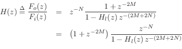
The final factored form above corresponds to the final equivalent form shown in Fig.6.17.
Related Forms
We see from the preceding example that a filtered-delay loop (a
feedback comb-filter using filtered feedback, with delay-line length
![]() in the above example) simulates a vibrating string in a manner
that is independent of where the excitation is applied. To
simulate the effect of a particular excitation point, a feedforward
comb-filter may be placed in series with the filtered delay loop.
Such a ``pluck position'' illusion may be applied to any basic string
synthesis algorithm, such as the EKS [428,207].
in the above example) simulates a vibrating string in a manner
that is independent of where the excitation is applied. To
simulate the effect of a particular excitation point, a feedforward
comb-filter may be placed in series with the filtered delay loop.
Such a ``pluck position'' illusion may be applied to any basic string
synthesis algorithm, such as the EKS [428,207].
By an exactly analogous derivation, a single feedforward comb filter can be used to simulate the location of a linearized magnetic pickup [200] on a simulated electric guitar string. An ideal pickup is formally the transpose of an excitation. For a discussion of filter transposition (using Mason's gain theorem [301,302]), see, e.g., [333,449].7.9
The comb filtering can of course also be implemented after the filtered delay loop, again by commutativity. This may be desirable in situations in which comb filtering is one of many options provided for in the ``effects section'' of a synthesizer. Post-processing comb filters are often used in reverberator design and in virtual pickup simulation.
![\includegraphics[width=\twidth]{eps/pianoSecondStringTap}](http://www.dsprelated.com/josimages_new/pasp/img1467.png) |
The comb-filtering can also be conveniently implemented using a second
tap from the appropriate delay element in the filtered delay loop
simulation of the string, as depicted in
Fig.6.18. The new tap output is simply
summed (or differenced, depending on loop implementation) with the
filtered delay loop output. Note that making the new tap a moving,
interpolating tap (e.g., using linear interpolation), a flanging
effect is available. The tap-gain ![]() can be brought out as a
musically useful timbre control that goes beyond precise physical
simulation (e.g., it can be made negative). Adding more moving taps
and summing/differencing their outputs, with optional scale factors,
provides an economical chorus or Leslie effect. These
extra delay effects cost no extra memory since they utilize the memory
that's already needed for the string simulation. While such effects
are not traditionally applied to piano sounds, they are applied to
electric piano sounds which can also be simulated using the same basic
technique.
can be brought out as a
musically useful timbre control that goes beyond precise physical
simulation (e.g., it can be made negative). Adding more moving taps
and summing/differencing their outputs, with optional scale factors,
provides an economical chorus or Leslie effect. These
extra delay effects cost no extra memory since they utilize the memory
that's already needed for the string simulation. While such effects
are not traditionally applied to piano sounds, they are applied to
electric piano sounds which can also be simulated using the same basic
technique.
Summary
In summary, two feedforward comb filters and one feedback comb filter arranged in series (in any order) can be interpreted as a physical model of a vibrating string driven at one point along the string and observed at a different point along the string. The two feedforward comb-filter delays correspond to the excitation and pickup locations along the string, while the amount of feedback-loop delay controls the fundamental frequency of vibration. A filter in the feedback loop determines the decay rate and fine tuning of the partial overtones.
Next Section:
General Loop-Filter Design
Previous Section:
Stiff String Synthesis Models


