


FDN Reverberation
Feedback Delay Networks (FDN) were introduced earlier in §2.7.
An example is shown in Fig.2.29 on page ![]() . After a
brief historical summary, this section will cover some practical
considerations for the use of FDNs as reverberators.
. After a
brief historical summary, this section will cover some practical
considerations for the use of FDNs as reverberators.
History of FDNs for Artificial Reverberation
Feedback delay networks were first suggested for artificial reverberation by Gerzon [156], who proposed an ``orthogonal matrix feedback reverberation unit''. He noted that individual feedback comb filters yielded poor quality, but that several such filters could sound good when cross-coupled. An ``orthogonal matrix feedback'' around a parallel bank of delay lines was suggested as a means of obtaining maximally rich cross-coupling. He was especially concerned with good stereo spreading of the reverberation at a time when most artificial reverberators sought merely to decorrelate the reverberation in each output channel.
Later, and apparently independently, Stautner and Puckette [473] suggested a specific four-channel FDN reverberator and gave general stability conditions for the FDN. They proposed the feedback matrix
![$\displaystyle \mathbf{A}= g\frac{1}{\sqrt{2}}
\left[\begin{array}{rrrr}
0 & 1 &...
... 0 \\
-1 & 0 & 0 & -1\\
1 & 0 & 0 & -1\\
0 & 1 & -1 & 0
\end{array}\right]
$](http://www.dsprelated.com/josimages_new/pasp/img744.png)
More recently, Jot [217,216] developed a systematic FDN design methodology allowing largely independent setting of reverberation time in different frequency bands. Using Jot's methodology, FDN reverberators can be polished to a high degree of quality, and they are presently considered to be among the best choices for high-quality artificial reverberation.
Jot's early work was concerned only with single-input, single-output (SISO) reverberators. Later work [218] with Jullien and others at IRCAM was concerned also with spatializing the reverberation.
![\includegraphics[width=\twidth]{eps/FDNJot}](http://www.dsprelated.com/josimages_new/pasp/img746.png)
An example FDN reverberator using three delay lines is shown in
Fig.3.10. It can be seen as an FDN (introduced in §2.7),
plus an additional low-order filter ![]() applied to the non-direct
signal. This filter is called a ``tonal correction'' filter by Jot,
and it serves to equalize modal energy irrespective of the
reverberation time in each band. In other words, if the decay time is
made very short in some band,
applied to the non-direct
signal. This filter is called a ``tonal correction'' filter by Jot,
and it serves to equalize modal energy irrespective of the
reverberation time in each band. In other words, if the decay time is
made very short in some band, ![]() will have a large gain in that
band so that the total energy in the band's impulse-response is
unchanged. This is another example of orthogonalization of
reverberation parameters: In this case, adjustments in reverberation
time, in any frequency band, do not alter total signal energy in the
impulse response in that band.
will have a large gain in that
band so that the total energy in the band's impulse-response is
unchanged. This is another example of orthogonalization of
reverberation parameters: In this case, adjustments in reverberation
time, in any frequency band, do not alter total signal energy in the
impulse response in that band.
Choice of Lossless Feedback Matrix
As mentioned in §3.4, an ``ideal'' late reverberation impulse response should resemble exponentially decaying noise [314]. It is therefore useful when designing a reverberator to start with an infinite reverberation time (the ``lossless case'') and work on making the reverberator a good ``noise generator''. Such a starting point is ofen referred to as a lossless prototype [153,430]. Once smooth noise is heard in the impulse response of the lossless prototype, one can then work on obtaining the desired reverberation time in each frequency band (as will be discussed in §3.7.4 below).
In reverberators based on feedback delay networks (FDNs), the smoothness of the ``perceptually white noise'' generated by the impulse response of the lossless prototype is strongly affected by the choice of FDN feedback matrix as well as the (ideally mutually prime) delay-line lengths in the FDN (discussed further in §3.7.3 below). Following are some of the better known feedback-matrix choices.
Hadamard Matrix
A second-order Hadamard matrix may be defined by
![$\displaystyle \mathbf{H}_2 \isdef
\frac{1}{\sqrt{2}}
\left[\begin{array}{rr}
1 & 1\\
-1 & 1
\end{array}\right],
$](http://www.dsprelated.com/josimages_new/pasp/img748.png)
![$\displaystyle \mathbf{H}_4 \isdef
\frac{1}{\sqrt{2}}
\left[\begin{array}{rr}
\...
...}{rrrr}
1& 1& 1&1\\
-1& 1&-1&1\\
-1&-1& 1&1\\
1&-1&-1&1
\end{array}\right].
$](http://www.dsprelated.com/josimages_new/pasp/img749.png)
As of version 0.9.30, Faust's math.lib4.12contains a function called hadamard(n) for generating an
![]() Hadamard matrix, where
Hadamard matrix, where ![]() must be a power of
must be a power of ![]() . A
Hadamard feedback matrix is used in the programming example
reverb_designer.dsp (a configurable FDN reverberator)
distributed with Faust.
. A
Hadamard feedback matrix is used in the programming example
reverb_designer.dsp (a configurable FDN reverberator)
distributed with Faust.
A Hadamard feedback matrix is said to be used in the IRCAM Spatialisateur [218].
Householder Feedback Matrix
One choice of lossless feedback matrix
![]() for FDNs, especially
nice in the
for FDNs, especially
nice in the ![]() case, is a specific Householder
reflection proposed by Jot [217]:
case, is a specific Householder
reflection proposed by Jot [217]:
where
It is interesting to note that when ![]() is a power of 2, no multiplies
are required [430]. For other
is a power of 2, no multiplies
are required [430]. For other ![]() , only one multiply is
required (by
, only one multiply is
required (by ![]() ).
).
Another interesting property of the Householder reflection
![]() given by Eq.
given by Eq.![]() (3.4) (and its permuted forms) is that an
(3.4) (and its permuted forms) is that an ![]() matrix-times-vector operation may be carried out with only
matrix-times-vector operation may be carried out with only ![]() additions (by first forming
additions (by first forming ![]() times the input vector, applying
the scale factor
times the input vector, applying
the scale factor ![]() , and subtracting the result from the input
vector). This is the same computation as physical wave
scattering at a junction of identical waveguides (§C.8).
, and subtracting the result from the input
vector). This is the same computation as physical wave
scattering at a junction of identical waveguides (§C.8).
An example implementation of a Householder FDN for ![]() is shown in
Fig.3.11. As observed by Jot [153, p.
216], this computation is equivalent to
is shown in
Fig.3.11. As observed by Jot [153, p.
216], this computation is equivalent to ![]() parallel feedback comb filters with one new feedback path from the
output to the input through a gain of
parallel feedback comb filters with one new feedback path from the
output to the input through a gain of ![]() .
.
![\includegraphics[width=0.7\twidth]{eps/householder1}](http://www.dsprelated.com/josimages_new/pasp/img762.png)
A nice feature of the Householder feedback matrix ![]() is that
for
is that
for ![]() , all entries in the matrix are nonzero. This
means every delay line feeds back to every other delay line, thereby
helping to maximize echo density as soon as possible.
, all entries in the matrix are nonzero. This
means every delay line feeds back to every other delay line, thereby
helping to maximize echo density as soon as possible.
Furthermore, for ![]() , all matrix entries have the same
magnitude:
, all matrix entries have the same
magnitude:
![$\displaystyle \mathbf{A}_4 = \frac{1}{2}
\left[\begin{array}{rrrr}
1 & -1 & -1 ...
...
-1 & 1 & -1 & -1\\
-1 & -1 & 1 & -1\\
-1 & -1 & -1 & 1
\end{array}\right].
$](http://www.dsprelated.com/josimages_new/pasp/img766.png)
Due to the elegant balance of the ![]() Householder feedback matrix,
Jot [216] proposes an
Householder feedback matrix,
Jot [216] proposes an ![]() FDN based on an embedding of
FDN based on an embedding of ![]() feedback matrices:
feedback matrices:
![$\displaystyle \mathbf{A}_{16} = \frac{1}{2}
\left[\begin{array}{rrrr}
\mathbf{A...
...\mathbf{A}_4 & -\mathbf{A}_4 & -\mathbf{A}_4 & \mathbf{A}_4
\end{array}\right]
$](http://www.dsprelated.com/josimages_new/pasp/img768.png)
Householder Reflections
For completeness, this section derives the Householder reflection
matrix from geometric considerations [451]. Let
![]() denote
the projection matrix which orthogonally projects vectors onto
denote
the projection matrix which orthogonally projects vectors onto
![]() , i.e.,
, i.e.,

Most General Lossless Feedback Matrices
As shown in §C.15.3, an FDN feedback matrix
![]() is
lossless if and only if its eigenvalues have modulus 1 and its
is
lossless if and only if its eigenvalues have modulus 1 and its ![]() eigenvectors are linearly independent.
eigenvectors are linearly independent.
A unitary matrix ![]() is any (complex) matrix that is inverted
by its own (conjugate) transpose:
is any (complex) matrix that is inverted
by its own (conjugate) transpose:
All unitary (and orthogonal) matrices have unit-modulus eigenvalues and linearly independent eigenvectors. As a result, when used as a feedback matrix in an FDN, the resulting FDN will be lossless (until the delay-line damping filters are inserted, as discussed in §3.7.4 below).
Triangular Feedback Matrices
An interesting class of feedback matrices, also explored by Jot [216], is that of triangular matrices. A basic fact from linear algebra is that triangular matrices (either lower or upper triangular) have all of their eigenvalues along the diagonal.4.13 For example, the matrix
![$\displaystyle \mathbf{A}_3 = \left[\begin{array}{ccc}
\lambda_1 & 0 & 0\\ [2pt]
a & \lambda_2 & 0\\ [2pt]
b & c & \lambda_3
\end{array}\right]
$](http://www.dsprelated.com/josimages_new/pasp/img786.png)
It is important to note that not all triangular matrices are lossless. For example, consider
![$\displaystyle \mathbf{A}_2 = \left[\begin{array}{cc} 1 & 0 \\ [2pt] 1 & 1 \end{array}\right]
$](http://www.dsprelated.com/josimages_new/pasp/img790.png)
![$\displaystyle \mathbf{A}_2^n = \left[\begin{array}{cc} 1 & 0 \\ [2pt] n & 1 \end{array}\right]
$](http://www.dsprelated.com/josimages_new/pasp/img793.png)
One way to avoid ``coupled repeated poles'' of this nature is to use
non-repeating eigenvalues. Another is to convert
![]() to Jordan
canonical form by means of a similarity transformation, zero any
off-diagonal elements, and transform back [329].
to Jordan
canonical form by means of a similarity transformation, zero any
off-diagonal elements, and transform back [329].
Choice of Delay Lengths
Following Schroeder's original insight, the delay line lengths in an
FDN (![]() in Fig.3.10) are typically chosen to be mutually
prime. That is, their prime factorizations contain no common
factors. This rule maximizes the number of samples that the lossless
reverberator prototype must be run before the impulse response
repeats.
in Fig.3.10) are typically chosen to be mutually
prime. That is, their prime factorizations contain no common
factors. This rule maximizes the number of samples that the lossless
reverberator prototype must be run before the impulse response
repeats.
The delay lengths ![]() should be chosen to ensure a
sufficiently high mode density in all frequency bands. An
insufficient mode density can be heard as ``ringing tones'' or an
uneven amplitude modulation in the late reverberation impulse
response.
should be chosen to ensure a
sufficiently high mode density in all frequency bands. An
insufficient mode density can be heard as ``ringing tones'' or an
uneven amplitude modulation in the late reverberation impulse
response.
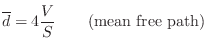
Mean Free Path
A rough guide to the average delay-line length is the ``mean free path'' in the desired reverberant environment. The mean free path is defined as the average distance a ray of sound travels before it encounters an obstacle and reflects. An approximate value for the mean free path, due to Sabine, an early pioneer of statistical room acoustics, is
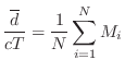
Mode Density Requirement
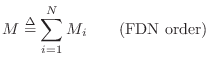
A guide for the sum of the delay-line lengths is the desired
mode density. The sum of delay-line lengths ![]() in a lossless
FDN is simply the order of the system
in a lossless
FDN is simply the order of the system ![]() :
:
Since the order of a system equals the number of poles, we have that
![]() is the number of poles on the unit circle in the lossless
prototype. If the modes were uniformly distributed, the mode density
would be
is the number of poles on the unit circle in the lossless
prototype. If the modes were uniformly distributed, the mode density
would be ![]() modes per Hz. Schroeder [417]
suggests that, for a reverberation time of 1 second, a mode density of
0.15 modes per Hz is adequate. Since the mode widths are inversely
proportional to reverberation time, the mode density for a
reverberation time of 2 seconds should be 0.3 modes per Hz, etc. In
summary, for a sufficient mode density in the frequency domain,
Schroeder's formula is
modes per Hz. Schroeder [417]
suggests that, for a reverberation time of 1 second, a mode density of
0.15 modes per Hz is adequate. Since the mode widths are inversely
proportional to reverberation time, the mode density for a
reverberation time of 2 seconds should be 0.3 modes per Hz, etc. In
summary, for a sufficient mode density in the frequency domain,
Schroeder's formula is
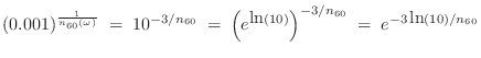
Prime Power Delay-Line Lengths
When the delay-line lengths need to be varied in real time, or
interactively in a GUI, it is convenient to choose each delay-line
length ![]() as an integer power of a distinct prime number
as an integer power of a distinct prime number ![]() [457]:
[457]:
Suppose we are initially given desired delay-line lengths ![]() arranged in ascending order so that
arranged in ascending order so that
![$\displaystyle \left[\frac{\log(M_i)}{\log(p_i)}\right]
\isdefs \left\lfloor 0.5 + \frac{\log(M_i)}{\log(p_i)}\right\rfloor.
$](http://www.dsprelated.com/josimages_new/pasp/img808.png)
This prime-power length scheme is used to keep 16 delay lines both variable and mutually prime in Faust's reverb_designer.dsp programming example (via the function prime_power_delays in effect.lib).
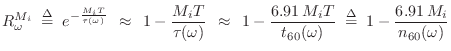
Achieving Desired Reverberation Times
A lossless prototype reverberator, as in Fig.3.10 when ![]() ,
has all of its poles on the unit circle in the
,
has all of its poles on the unit circle in the ![]() plane, and its
reverberation time is infinity. To set the reverberation time to a
desired value, we need to move the poles slightly inside the unit
circle. Furthermore, due to air absorption
(§2.3,§B.7.15), we want the high-frequency
poles to be more damped than the low-frequency poles
[314]. As discussed in §2.3, this type
of transformation can be obtained using the substitution
plane, and its
reverberation time is infinity. To set the reverberation time to a
desired value, we need to move the poles slightly inside the unit
circle. Furthermore, due to air absorption
(§2.3,§B.7.15), we want the high-frequency
poles to be more damped than the low-frequency poles
[314]. As discussed in §2.3, this type
of transformation can be obtained using the substitution
where
Solving for
The last form comes from
Series expanding
Conformal Map Interpretation of Damping Substitution
The relation
![]() [Eq.
[Eq.![]() (3.7)] can
be written down directly from
(3.7)] can
be written down directly from
![]() [Eq.
[Eq.![]() (3.5)] by interpreting Eq.
(3.5)] by interpreting Eq.![]() (3.5) as an approximate
conformal map [326] which takes each pole
(3.5) as an approximate
conformal map [326] which takes each pole
![]() ,
say, from the unit circle to the point
,
say, from the unit circle to the point
![]() .
Thus, the new pole radius is approximately
.
Thus, the new pole radius is approximately
![]() ,
where the approximation is valid when
,
where the approximation is valid when ![]() is approximately constant
between the new pole location and the unit circle. To see this,
consider the partial fraction expansion [449] of a proper
is approximately constant
between the new pole location and the unit circle. To see this,
consider the partial fraction expansion [449] of a proper
![]() th-order lossless transfer function
th-order lossless transfer function ![]() mapped to
mapped to
![]() :
:
![$\displaystyle H'(z)
= \sum_{k=1}^N \frac{r_k}{1-p_kG(z)z^{-1}}
= \sum_{k=1}^N r_k\left[1+p_kG(z)z^{-1}+p_k^2G^2(z)z^{-2}+\cdots\right],
$](http://www.dsprelated.com/josimages_new/pasp/img838.png)
Happily, while we may not know precisely where our poles have moved as
a result of introducing the per-sample damping filter ![]() , the
relation
, the
relation
![]() [Eq.
[Eq.![]() (3.6)] remains
exact at every frequency by construction, as it is based only on the
physical interpretation of each unit delay as a propagation delay for
a plane wave across one sampling interval
(3.6)] remains
exact at every frequency by construction, as it is based only on the
physical interpretation of each unit delay as a propagation delay for
a plane wave across one sampling interval ![]() , during which
(zero-phase) filtering by
, during which
(zero-phase) filtering by ![]() is assumed (§2.3). More
generally, we can design minimum-phase filters for which
is assumed (§2.3). More
generally, we can design minimum-phase filters for which
![]() , and neglect the resulting
phase dispersion.
, and neglect the resulting
phase dispersion.
In summary, we see that replacing ![]() by
by
![]() everywhere in the
FDN lossless prototype (or any lossless LTI system for that matter)
serves to move its poles away from the unit circle in the
everywhere in the
FDN lossless prototype (or any lossless LTI system for that matter)
serves to move its poles away from the unit circle in the ![]() plane
onto some contour inside the unit circle that provides the desired
decay time at each frequency.
plane
onto some contour inside the unit circle that provides the desired
decay time at each frequency.
A general design guideline for artificial reverberation applications
[217] is that all pole radii in the
reverberator should vary smoothly with frequency. This translates
to ![]() having a smooth frequency response. To see why this
is desired, consider momentarily the frequency-independent case in
which we desire the same reverberation time at all frequencies
(Fig.3.10 with real
having a smooth frequency response. To see why this
is desired, consider momentarily the frequency-independent case in
which we desire the same reverberation time at all frequencies
(Fig.3.10 with real ![]() , as drawn). In this case, it is
ideal for all of the poles to have this decay time. Otherwise, the
late decay of the impulse response will be dominated by the poles
having the largest magnitude, and it will be ``thinner'' than it was
at the beginning of the response when all poles were contributing to
the output. Only when all poles have the same magnitude will the late
response maintain the same modal density throughout the decay.
, as drawn). In this case, it is
ideal for all of the poles to have this decay time. Otherwise, the
late decay of the impulse response will be dominated by the poles
having the largest magnitude, and it will be ``thinner'' than it was
at the beginning of the response when all poles were contributing to
the output. Only when all poles have the same magnitude will the late
response maintain the same modal density throughout the decay.
Damping Filters for Reverberation Delay Lines
In an FDN, such as the one shown in Fig.3.10, delays ![]() appear
in long delay-line chains
appear
in long delay-line chains ![]() . Therefore, the filter needed at
the output (or input) of the
. Therefore, the filter needed at
the output (or input) of the ![]() th delay line is
th delay line is
![]() (replace
(replace
![]() by
by
![]() in Fig.3.10).4.15 However, because
in Fig.3.10).4.15 However, because
![]() is so close to
is so close to ![]() in magnitude, and because it varies so weakly
across the frequency axis, we can design a much lower-order filter
in magnitude, and because it varies so weakly
across the frequency axis, we can design a much lower-order filter
![]() that provides the desired attenuation
versus frequency to within psychoacoustic resolution. In fact,
perfectly nice reverberators can be designed in which
that provides the desired attenuation
versus frequency to within psychoacoustic resolution. In fact,
perfectly nice reverberators can be designed in which ![]() is
merely first order for each
is
merely first order for each ![]() [314,217].
[314,217].
Delay-Line Damping Filter Design
Let
![]() denote the desired reverberation time at radian frequency
denote the desired reverberation time at radian frequency
![]() , and let
, and let ![]() denote the transfer function of the lowpass
filter to be placed in series with the
denote the transfer function of the lowpass
filter to be placed in series with the ![]() th delay line which is
th delay line which is ![]() samples long. The problem we consider now is how to design these
filters to yield the desired reverberation time. We will specify an
ideal amplitude response for
samples long. The problem we consider now is how to design these
filters to yield the desired reverberation time. We will specify an
ideal amplitude response for ![]() based on the desired
reverberation time at each frequency, and then use conventional
filter-design methods to obtain a low-order approximation to this
ideal specification.
based on the desired
reverberation time at each frequency, and then use conventional
filter-design methods to obtain a low-order approximation to this
ideal specification.
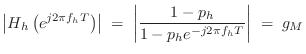
In accordance with Eq.![]() (3.6), the lowpass filter
(3.6), the lowpass filter ![]() in series
with a length
in series
with a length ![]() delay line should approximate
delay line should approximate
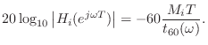
This is the same formula derived by Jot [217] using a somewhat different approach.
Now that we have specified the ideal delay-line filter
![]() in
terms of its amplitude response in dB, any number of filter-design
methods can be used to find a low-order
in
terms of its amplitude response in dB, any number of filter-design
methods can be used to find a low-order ![]() which provides a good
approximation to satisfying Eq.
which provides a good
approximation to satisfying Eq.![]() (3.9). Examples include the functions
invfreqz and stmcb in Matlab. Since the variation
in reverberation time is typically very smooth with respect to
(3.9). Examples include the functions
invfreqz and stmcb in Matlab. Since the variation
in reverberation time is typically very smooth with respect to
![]() , the filters
, the filters ![]() can be very low order.
can be very low order.
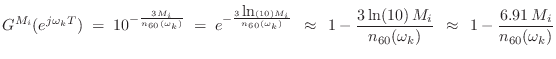
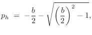
First-Order Delay-Filter Design
The first-order case is very simple while enabling separate control of
low-frequency and high-frequency reverberation times. For simplicity,
let's specify ![]() and
and
![]() , denoting the desired
decay-time at dc (
, denoting the desired
decay-time at dc (![]() ) and half the sampling rate
(
) and half the sampling rate
(
![]() ). Then we have determined the coefficients of a
one-pole filter:
). Then we have determined the coefficients of a
one-pole filter:
![\begin{eqnarray*}
\frac{g_i}{1-p_i} &=& 10^{-3 M_i T / t_{60}(0)}
\eqsp e^{-M_iT...
...(\pi/T)}
\eqsp e^{-M_iT/\tau(\pi/T)} \isdefs R_\pi^{M_i}\\ [5pt]
\end{eqnarray*}](http://www.dsprelated.com/josimages_new/pasp/img870.png)
where
![]() denotes the
denotes the ![]() th delay-line length in
seconds. These two equations are readily solved to yield
th delay-line length in
seconds. These two equations are readily solved to yield
![\begin{eqnarray*}
p_i &=& \frac{R_0^{M_i}-R_\pi^{M_i}}{R_0^{M_i}+R_\pi^{M_i}}\\ [5pt]
g_i &=& \frac{2R_0^{M_i}R_\pi^{M_i}}{R_0^{M_i}+R_\pi^{M_i}}
\end{eqnarray*}](http://www.dsprelated.com/josimages_new/pasp/img872.png)
The truncated series approximation
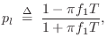
Orthogonalized First-Order Delay-Filter Design
In [217], first-order delay-line filters of the form

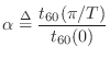
denotes the ratio of reverberation time at half the sampling rate divided by the reverberation time at dc.4.16
Multiband Delay-Filter Design
In §3.7.5, we derived first-order FDN delay-line filters which
can independently set the reverberation time at dc and at half the
sampling rate. However, perceptual studies indicate that
reverberation time should be independently adjustable in at least
three frequency bands [217]. To provide this degree
of control (and more), one can implement a multiband delay-line filter
using a general-purpose filter bank
[370,500]. The output, say, of each delay
line is split into ![]() bands, where
bands, where ![]() is recommended, and then,
from Eq.
is recommended, and then,
from Eq.![]() (3.6), the gain in the
(3.6), the gain in the ![]() th band for a length
th band for a length ![]() delay-line can be set to
delay-line can be set to
Spectral Coloration Equalizer
In the previous section, a ``graphical equalizer'' was used to set the
reverberator decay time independently in each spectral band slice.
While this gives much control over decay time, there is no control
over the initial spectral gain in each band. Therefore, another good
place for a graphical equalizer is at the reverberator input or
output. Such an equalizer allows control of the initial
spectral coloration of the reverberator. In the example of
Fig.3.10, a spectral coloration equalizer is most efficiently
applied to the input signal ![]() , before entering the FDN (but after
splitting off the direct signal to be scaled by
, before entering the FDN (but after
splitting off the direct signal to be scaled by ![]() and added to the
output), or the output of
and added to the
output), or the output of ![]() in Fig.3.10.
in Fig.3.10.
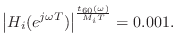
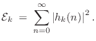
Tonal Correction Filter
Let ![]() denote the component of the impulse response arising from
the
denote the component of the impulse response arising from
the ![]() th pole of the system. Then the energy associated with that pole
is
th pole of the system. Then the energy associated with that pole
is
In the case of the first-order delay-line filters discussed in §3.7.5, good tonal correction is given by the following one-zero filter:

FDNs as Digital Waveguide Networks
As discussed in §C.15, the FDN using a
Householder-reflection feedback matrix
![]() is equivalent to a network of
is equivalent to a network of ![]() digital waveguides
intersecting at a single scattering junction
[463,464,385]. The wave impedance in the
digital waveguides
intersecting at a single scattering junction
[463,464,385]. The wave impedance in the ![]() th
waveguide is simply
th
waveguide is simply
![]() , the
, the ![]() th element of the
axis-of-reflection vector
th element of the
axis-of-reflection vector
![]() . The choice
. The choice
![]() corresponds to all of the waveguides having the same impedance (the
``isotrophic junction'' case).
corresponds to all of the waveguides having the same impedance (the
``isotrophic junction'' case).
FDN Reverberators in Faust
The Faust example reverb_designer.dsp brings up a
![]() FDN reverberator in which the signal out of each delay line is
split into five bands so that
FDN reverberator in which the signal out of each delay line is
split into five bands so that
![]() can be controlled
independently in each band. The 16 delay-line lengths are distributed
exponentially between a minimum and maximum length set by two
min/max-length sliders, but rounded to the nearest integer-power of a
distinct prime, as introduced above in §3.7.3). The FDN
reverberator is implemented in Faust's effect.lib. The
band-splitting is carried out by the filterbank function in
Faust's filter.lib.
can be controlled
independently in each band. The 16 delay-line lengths are distributed
exponentially between a minimum and maximum length set by two
min/max-length sliders, but rounded to the nearest integer-power of a
distinct prime, as introduced above in §3.7.3). The FDN
reverberator is implemented in Faust's effect.lib. The
band-splitting is carried out by the filterbank function in
Faust's filter.lib.
The Faust function filterbank(order,freqs) implements a filter bank having the needed properties using Butterworth lowpass/highpass band-splitting arranged in a dyadic tree (normally a good choice for audio filter banks). That is, the whole spectrum is split at the highest crossover frequency, the lowpass region is then split into two bands at the next crossover frequency down, and so on, splitting the lowpass band at each stage in the dyadic tree [455,500]. The number of poles in each Butterworth lowpass/highpass filter is specified by order, and freqs contains a list of desired crossover frequencies separating the bands. A certain amount of dispersion is also introduced, since the filter bank is causal and delay-equalized (so that the bands may be summed without phase cancellation artifacts at the band edges). Also note that the lower bands are effectively produced by higher order filters than the upper bands. When the reverberation time is longer than the dispersion delay, the dispersion should not be audible as such, although it can affect the ``sound'' of the reverberation. In general, however, artificial reverberators normally benefit from additional allpass dispersion.
Figure 3.12 shows the block diagram of a ![]() FDN
reverberator made from Faust's reverb_designer.dsp by
changing 16 to 4. Figure 3.13 shows the Faust block diagram of
the associated
FDN
reverberator made from Faust's reverb_designer.dsp by
changing 16 to 4. Figure 3.13 shows the Faust block diagram of
the associated ![]() Hamard matrix multiplication. As it shows,
multiplication by a Hadamard matrix can be implemented (ignoring the
normalizing scale factor) as a series of block sums and differences
(often called butterflies or shufflers) in which the
block size decreases by a factor of 2 each stage. Figures for the
remaining components of the reverberator may be perused via the shell
command faust2firefox reverb_designer.dsp followed by
clicking on the blocks in the browser.
Hamard matrix multiplication. As it shows,
multiplication by a Hadamard matrix can be implemented (ignoring the
normalizing scale factor) as a series of block sums and differences
(often called butterflies or shufflers) in which the
block size decreases by a factor of 2 each stage. Figures for the
remaining components of the reverberator may be perused via the shell
command faust2firefox reverb_designer.dsp followed by
clicking on the blocks in the browser.
![\includegraphics[width=\twidth]{eps/fdnrev0}](http://www.dsprelated.com/josimages_new/pasp/img894.png) |
![\includegraphics[width=\twidth]{eps/hadamard4}](http://www.dsprelated.com/josimages_new/pasp/img895.png)
Zita-Rev1
A FOSS4.17 reverberator that combines elements of Schroeder (§3.5) and FDN reverberators (§3.7) is zita-rev1,4.18written in C++ for Linux systems by Fons Adriaensen. A Faust version of the zita-rev1 stereo-mode functionality is zita_rev1 in Faust's effect.lib. A high-level block diagram appears in Fig.3.14.
![\includegraphics[width=\twidth]{eps/zita-rev1}](http://www.dsprelated.com/josimages_new/pasp/img897.png) |
The main high-level addition relative to an 8th-order FDN reverberator
is the block labeled allpass_combs in Fig.3.14.
This block inserts a Schroeder allpass comb filter (Fig.2.30) in
series with each delay line. In zita-rev1 (as of this
writing), the allpass-comb feedforward/feedback coefficients are all
set to ![]() . The delay-line lengths and other details are readily
found in the freely available source code (or by browsing the
Faust-generated block diagram).
. The delay-line lengths and other details are readily
found in the freely available source code (or by browsing the
Faust-generated block diagram).
Zita-Rev1 Delay-Line Filters
In zita-rev1, the damping filter for each delay line consists
of a low-shelf filter ![]() [449],4.19in series with a unique first-order lowpass filter
[449],4.19in series with a unique first-order lowpass filter ![]() that sets
the high-frequency
that sets
the high-frequency ![]() to be half that of the middle-band at a
particular frequency
to be half that of the middle-band at a
particular frequency ![]() (specified as ``HF Damping'' in the GUI).
Since the filter
(specified as ``HF Damping'' in the GUI).
Since the filter ![]() is constrained to be a lowpass,
is constrained to be a lowpass,
![]() for
for ![]() , i.e., the decay time gets
shorter at higher frequencies.
, i.e., the decay time gets
shorter at higher frequencies.
Viewing the resulting damping filter
![]() as a
three-band filter bank (§3.7.5), let
as a
three-band filter bank (§3.7.5), let ![]() and
and ![]() denote the
desired band gains at dc and ``middle frequencies'',
respectively.4.20 Then the low shelf may be set for a
desired dc-gain of
denote the
desired band gains at dc and ``middle frequencies'',
respectively.4.20 Then the low shelf may be set for a
desired dc-gain of ![]() , and its input (or output) signal
multiplied by
, and its input (or output) signal
multiplied by ![]() to obtain the resulting filter
to obtain the resulting filter

The lowpass filter ![]() is also first order, and to provide half
the middle-band
is also first order, and to provide half
the middle-band ![]() at the beginning of the ``high'' band, the
lowpass should ``break'' to a gain of
at the beginning of the ``high'' band, the
lowpass should ``break'' to a gain of ![]() at the ``HF Damping''
frequency
at the ``HF Damping''
frequency ![]() specified in the GUI. A unity-dc-gain one-pole
lowpass has the form [449]
specified in the GUI. A unity-dc-gain one-pole
lowpass has the form [449]

Further Extensions
Schroeder's original structures for artificial reverberation were comb filters and allpass filters made from two comb filters. Since then, they have been upgraded to include specific early reflections and per-sample air-absorption filtering (Moorer, Schroeder), precisely specified frequency dependent reverberation time (Jot), and a nearly independent factorization of ``coloration'' and ``duration'' aspects (Jot). The evolution from comb filters to feedback delay networks (Gerzon, Stautner, Puckette, Jot) can be seen as a means for obtaining greater richness of feedback, so that the diffuseness of the impulse response is greater than what is possible with parallel and/or series comb filters. In fact, an FDN can be seen as a richly cross-coupled bank of feedback comb filters whenever the diagonal of the feedback matrix is nonzero. The question then becomes what aspects of artificial reverberation have not yet been fully addressed?
Spatialization of Reverberant Reflections
While we did not go into the subject here, the early reflections should be spatialized by including a head-related transfer function (HRTF) on each tap of the early-reflection delay line [248].4.21
Some kind of spatialization may be needed also for the late reverberation. A true diffuse field (§3.2.1) consists of a sum of plane waves traveling in all directions in 3D space. Since we do not know how to achieve this effect using current systems for reverberation, the typical goal is to simply extract uncorrelated outputs from the reverberation network and feed them to the various output channels, as discussed in §3.5. However, this is not ideal, since the resulting sound field consists of wavefronts arriving from each of the speakers, and it is possible for the reverberation to sound like it is emanating from discrete speaker locations. It may be that spatialization of some kind can better fool the ear into believing the late reverberation is coming from all directions.
Distribution of Mode Frequencies
Another way in which current reverberation systems are ``artificial''
is the unnaturally uniform distribution of resonant modes with respect
to frequency. Because Schroeder, FDN, and waveguide reverbs are
all essentially a collection of ![]() delay lines with feedback around
them, the modes tend to be distributed as the superposition of the
resonant modes of
delay lines with feedback around
them, the modes tend to be distributed as the superposition of the
resonant modes of ![]() feedback comb filters. Since a feedback comb
filter has a nearly harmonic set of modes (see §2.6.2),
aggregates of comb filters tend to provide a uniform modal density in
the frequency domain. In real reverberant spaces, the mode density
increases as frequency squared, so it should be verified that the
uniform modes used in a reverberator are perceptually equivalent to
the increasingly dense modes in nature. Another aspect of perception
to consider is that frequency-domain perception of resonances actually
decreases with frequency. To summarize, in nature the modes get denser
with frequency, while in perception they are less resolved, and in
current reverberation systems they stay more or less uniform with
frequency; perhaps a uniform distribution is a good compromise between
nature and perception?
feedback comb filters. Since a feedback comb
filter has a nearly harmonic set of modes (see §2.6.2),
aggregates of comb filters tend to provide a uniform modal density in
the frequency domain. In real reverberant spaces, the mode density
increases as frequency squared, so it should be verified that the
uniform modes used in a reverberator are perceptually equivalent to
the increasingly dense modes in nature. Another aspect of perception
to consider is that frequency-domain perception of resonances actually
decreases with frequency. To summarize, in nature the modes get denser
with frequency, while in perception they are less resolved, and in
current reverberation systems they stay more or less uniform with
frequency; perhaps a uniform distribution is a good compromise between
nature and perception?
At low frequencies, however, resonant modes are accurately perceived in reverberation as boosts, resonances, and cuts. They are analogous to early reflections in the time domain, and we could call them the ``early resonances.'' It is interesting that no system for artificial reverberation except waveguide mesh reverberation (of which the author is aware) explicitly attempts precise shaping of the low-frequency amplitude response of a desired reverberant space, at least not directly. The low-frequency response is shaped indirectly by the choice of early reflections, and the use of parallel comb-filter banks in Schroeder reverberators serves also to shape the low-frequency response significantly. However, it would be possible to add filters for shaping more carefully the low-frequency response. Perhaps a reason for this omission is that hall designers work very hard to eliminate any explicit resonances or antiresonances in the response of a room. If uneven resonance at low frequencies is always considered a defect, then designing for a maximally uniform mode distribution, as has been discussed for the high-frequency modes, would be ideal also at low frequencies. Quite the opposite situation exists when designing ``small-box reverberators'' to simulate musical instrument resonators [428,203]; there, the low-frequency modes impart a characteristic timbre on the low-frequency resonance of the instrument (see Fig.3.2).
Digital Waveguide Reverberators
It was mentioned in §3.7.8 above that FDNs can be formulated as special cases of Digital Waveguide Networks (DWN) (see Appendix C for a fuller development of DWNs). Specifically, an FDN is obtained from a DWN consisting of a single scattering junction (§C.15). It follows that the DWN paradigm provides a more generalized framework in which to pursue further improvements of reverberation architecture. For example, when multiple FDNs are embedded within a single DWN, it becomes possible to richly cross-couple them in an energy-controlled manner in order to create richer recursive structures than either alone. General DWNs were proposed for artificial reverberation in [430,433].
The Digital Waveguide Mesh for Reverberation
A special case of digital waveguide networks known as the digital waveguide mesh has also been proposed for use in artificial reverberation systems [396,518].
As discussed in §2.4, a digital waveguide (bidirectional delay line) can be considered a computational acoustic model for traveling waves in opposite directions. A mesh of such waveguides in 2D or 3D can simulate waves traveling in any direction in the space. As an analogy, consider a tennis racket in which a rectilinear mesh of strings forms a pseudo-membrane.
A major advantage of the waveguide mesh for reverberation applications is that wavefronts are explicitly simulated in all directions, as in real reverberant spaces. Therefore, a true diffuse field can be developed in the late reverberation. Also, the echo density grows with time and the mode density grows with frequency in a natural manner for the 2D and 3D mesh. Finally, the low-frequency modes of the reverberant space can be simulated very precisely (for better or worse).
The computational cost of a waveguide mesh is made tractable relative to more conventional finite-difference simulations by (1) the use of multiply-free scattering junctions and (2) very coarse meshes. Use of a coarse mesh means that the ``physical modeling'' aspects of the mesh are only valid at low frequencies. As practical matter, this works out well because the ear cannot hear mode tuning errors at high frequencies. There is no error in the mode dampings in a lossless reverberator prototype, because the waveguide mesh is lossless by construction. Therefore, the only errors relative to an ideal simulation of a lossless membrane or space are (1) mode tuning error, and (2) finite band width (cut off at half the sampling rate). The tuning error can be understood as due to dispersion of the traveling waves in certain directions [518,399]. Much progress has been made on the problem of correcting this dispersion error in various mesh geometries (rectilinear, triangular, tetrahedral, etc.) [521,398,399].
See §C.14 for an introduction to the digital waveguide mesh and a few of its properties.
Time Varying Reverberators
In real rooms, thermal convention currents cause the propagation path delays to vary over time [58]. Therefore, for greater physical accuracy, the delay lines within a digital reverberator should vary over time. From a more practical perspective, time variation helps to break up and obscure unwanted repetition in the late reverberation impulse response [430,104].
Next Section:
Delay-Line Interpolation
Previous Section:
Freeverb


