


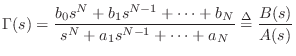
Lumped Models
This chapter introduces modeling of ``lumped'' physical systems, such as configurations of masses, springs, and ``dashpots''.The term ``lumped'' comes from electrical engineering, and refers to lumped-parameter analysis, as opposed to distributed-parameter analysis. Examples of ``distributed'' systems in musical acoustics include ideal strings, acoustic tubes, and anything that propagates waves. In general, a lumped-parameter approach is appropriate when the physical object has dimensions that are small relative to the wavelength of vibration. Examples from musical acoustics include brass-players' lips (modeled using one or two masses attached to springs--see §9.7), and the piano hammer (modeled using a mass and nonlinear spring, as discussed in §9.4). In contrast to these lumped-modeling examples, the vibrating string is most efficiently modeled as a sampled distributed-parameter system, as discussed in Chapter 6, although lumped models of strings (using, e.g., a mass-spring-chain [318]) work perfectly well, albeit at a higher computational expense for a given model quality [69,145]. In the realm of electromagnetism, distributed-parameter systems include electric transmission lines and optical waveguides, while the typical lumped-parameter systems are ordinary RLC circuits (connecting resistors, capacitors, and inductors). Again, whenever the oscillation wavelength is large relative to the geometry of the physical component, a lumped approximation may be considered. As a result, there is normally a high-frequency limit on the validity of a lumped-parameter model. For the same reason, there is normally an upper limit on physical size as well.
We begin with the fundamental concept of impedance, and discuss the elementary lumped impedances associated with springs, mass, and dashpots. These physical objects are analogous to capacitors, inductors, and resistors in lumped-parameter electrical circuits. Next, we discuss general interconnections of such elements, characterized at a single input/output location by means of one-port network theory. In particular, we will see that all passive networks present a positive real impedance at any port (input/output point). A network diagram may be replaced by an impedance diagram, which may then be translated into its equivalent circuit (replacing springs by capacitors, masses by inductors, and dashpots by resistors).
In the following chapter, we discuss digitization of lumped networks by various means, including finite differences and the bilinear transformation.
Impedance
Impedance is defined for mechanical systems as
force divided by velocity, while the inverse (velocity/force) is
called an admittance. For dynamic systems, the impedance of a
``driving point'' is defined for each frequency ![]() , so that the
``force'' in the definition of impedance is best thought of as the
peak amplitude of a sinusoidal applied force, and similarly for the
velocity. Thus, if
, so that the
``force'' in the definition of impedance is best thought of as the
peak amplitude of a sinusoidal applied force, and similarly for the
velocity. Thus, if ![]() denotes the Fourier transform of the
applied force at a driving point, and
denotes the Fourier transform of the
applied force at a driving point, and ![]() is the Fourier
transform of the resulting velocity of the driving point, then the
driving-point impedance is given by
is the Fourier
transform of the resulting velocity of the driving point, then the
driving-point impedance is given by
In acoustics [317,318], force takes the form of
pressure
(e.g., in physical units of newtons per meter squared),
and velocity may be either particle velocity in open air
(meters per second) or volume velocity in acoustic tubes
(meters cubed per second) (see §B.7.1 for
definitions).
The wave impedance (also called the characteristic
impedance) in open air is the ratio of pressure to particle velocity
in a sound wave traveling through air, and it is given by
![]() , where
, where ![]() is the density (mass
per unit volume) of air,
is the density (mass
per unit volume) of air, ![]() is the speed of sound propagation,
is the speed of sound propagation, ![]() is ambient pressure, and
is ambient pressure, and
![]() is the ratio of the specific
heat of air at constant pressure to that at constant volume. In a
vibrating string, the wave impedance is given by
is the ratio of the specific
heat of air at constant pressure to that at constant volume. In a
vibrating string, the wave impedance is given by
![]() , where
, where ![]() is string density (mass per unit length) and
is string density (mass per unit length) and ![]() is
the tension of the string (stretching force), as discussed further in
§C.1 and §B.5.2.
is
the tension of the string (stretching force), as discussed further in
§C.1 and §B.5.2.
In circuit theory [110], force takes the form of electric
potential in volts, and velocity manifests as electric current in amperes
(coulombs per second). In an electric transmission line, the
characteristic impedance is given by
![]() where
where ![]() and
and ![]() are the inductance and capacitance, respectively, per unit length along the
transmission line. In free space, the wave impedance for light is
are the inductance and capacitance, respectively, per unit length along the
transmission line. In free space, the wave impedance for light is
![]() , where
, where ![]() and
and
![]() are
the permeability and permittivity, respectively, of free space. One might
be led from this to believe that there must exist a medium, or `ether',
which sustains wave propagation in free space; however, this is one
instance in which ``obvious'' predictions from theory turn out to be wrong.
are
the permeability and permittivity, respectively, of free space. One might
be led from this to believe that there must exist a medium, or `ether',
which sustains wave propagation in free space; however, this is one
instance in which ``obvious'' predictions from theory turn out to be wrong.
Dashpot
The elementary impedance element in mechanics is the dashpot which
may be approximated mechanically by a plunger in a cylinder of air or
liquid, analogous to a shock absorber for a car. A constant impedance
means that the velocity produced is always linearly proportional to the
force applied, or
![]() , where
, where ![]() is the dashpot impedance,
is the dashpot impedance,
![]() is the applied force at time
is the applied force at time ![]() , and
, and ![]() is the velocity. A
diagram is shown in Fig. 7.1.
is the velocity. A
diagram is shown in Fig. 7.1.
![\includegraphics[scale=0.9]{eps/ldashpot}](http://www.dsprelated.com/josimages_new/pasp/img1569.png) |
In circuit theory, the element analogous to the dashpot is the
resistor ![]() , characterized by
, characterized by
![]() , where
, where ![]() is voltage
and
is voltage
and ![]() is current. In an analog equivalent circuit, a dashpot can be
represented using a resistor
is current. In an analog equivalent circuit, a dashpot can be
represented using a resistor ![]() .
.
Over a specific velocity range, friction force can also be
characterized by the relation
![]() . However, friction is
very complicated in general [419], and as the velocity goes
to zero, the coefficient of friction
. However, friction is
very complicated in general [419], and as the velocity goes
to zero, the coefficient of friction ![]() may become much larger.
The simple model often presented is to use a static coefficient
of friction when starting at rest (
may become much larger.
The simple model often presented is to use a static coefficient
of friction when starting at rest (![]() ) and a dynamic
coefficient of friction when in motion (
) and a dynamic
coefficient of friction when in motion (
![]() ). However, these
models are too simplified for many practical situations in musical
acoustics, e.g., the frictional force between the bow and string of a
violin [308,549], or the internal friction losses
in a vibrating string [73].
). However, these
models are too simplified for many practical situations in musical
acoustics, e.g., the frictional force between the bow and string of a
violin [308,549], or the internal friction losses
in a vibrating string [73].
Ideal Mass
![\includegraphics[scale=0.9]{eps/lmass}](http://www.dsprelated.com/josimages_new/pasp/img1575.png)
The concept of impedance extends also to masses and springs.
Figure 7.2 illustrates an ideal mass of ![]() kilograms
sliding on a frictionless surface. From Newton's second law of motion, we
know force equals mass times acceleration, or
kilograms
sliding on a frictionless surface. From Newton's second law of motion, we
know force equals mass times acceleration, or
Since impedance is defined in terms of force and velocity, we will prefer the
form
![]() . By the differentiation theorem for Laplace transforms
[284],8.1we have
. By the differentiation theorem for Laplace transforms
[284],8.1we have
Since we normally think of an applied force as an input and the resulting
velocity as an output, the corresponding transfer function is
![]() . The system diagram for this view
is shown in Fig. 7.3.
. The system diagram for this view
is shown in Fig. 7.3.
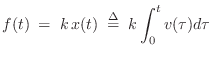
The impulse response of a mass, for a force input and velocity output, is defined as the inverse Laplace transform of the transfer function:
![\includegraphics[scale=0.9]{eps/lblackbox}](http://www.dsprelated.com/josimages_new/pasp/img1587.png) |
Once the input and output signal are defined, a transfer function is
defined, and therefore a frequency response is defined [485].
The frequency response is given by the transfer function evaluated on
the ![]() axis in the
axis in the ![]() plane, i.e., for
plane, i.e., for ![]() . For the ideal mass,
the force-to-velocity frequency response is
. For the ideal mass,
the force-to-velocity frequency response is
In circuit theory, the element analogous to the mass is the inductor,
characterized by
![]() , or
, or
![]() . In an analog
equivalent circuit, a mass can be represented using an inductor with value
. In an analog
equivalent circuit, a mass can be represented using an inductor with value
![]() .
.
Ideal Spring
Figure 7.4 depicts the ideal spring.
![\includegraphics[width=3in]{eps/lspring}](http://www.dsprelated.com/josimages_new/pasp/img1592.png)
From Hooke's law, we have that the applied force is proportional to the displacement of the spring:

The frequency response of the ideal spring, given the applied force as input and resulting velocity as output, is
In this case, the amplitude response grows
We call ![]() the compression velocity of the spring. In more
complicated configurations, the compression velocity is defined as the
difference between the velocity of the two spring endpoints, with positive
velocity corresponding to spring compression.
the compression velocity of the spring. In more
complicated configurations, the compression velocity is defined as the
difference between the velocity of the two spring endpoints, with positive
velocity corresponding to spring compression.
In circuit theory, the element analogous to the spring is the capacitor,
characterized by
![]() , or
, or
![]() .
In an equivalent analog circuit, we can use the value
.
In an equivalent analog circuit, we can use the value ![]() . The
inverse
. The
inverse ![]() of the spring stiffness is sometimes called the
compliance
of the spring.
of the spring stiffness is sometimes called the
compliance
of the spring.
Don't forget that the definition of impedance requires zero initial conditions for elements with ``memory'' (masses and springs). This means we can only use impedance descriptions for steady state analysis. For a complete analysis of a particular system, including the transient response, we must go back to full scale Laplace transform analysis.
One-Port Network Theory
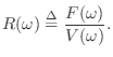
The basic idea of a one-port network [524] is shown in Fig. 7.5. The one-port is a ``black box'' with a single pair of input/output terminals, referred to as a port. A force is applied at the terminals and a velocity ``flows'' in the direction shown. The admittance ``seen'' at the port is called the driving point admittance. Network theory is normally described in terms of circuit theory elements, in which case a voltage is applied at the terminals and a current flows as shown. However, in our context, mechanical elements are preferable.
![\includegraphics[scale=0.9]{eps/loneport}](http://www.dsprelated.com/josimages_new/pasp/img1604.png) |
Series Combination of One-Ports
Figure 7.6 shows the series combination of two one-ports.
![\includegraphics[scale=0.9]{eps/lseries}](http://www.dsprelated.com/josimages_new/pasp/img1605.png)
Impedances add in series, so the aggregate impedance is
![]() , and the admittance is
, and the admittance is
Mass-Spring-Wall System
In a physical situation, if two elements are connected in such a way that they share a common velocity, then they are in series. An example is a mass connected to one end of a spring, where the other end is attached to a rigid support, and the force is applied to the mass, as shown in Fig. 7.7.
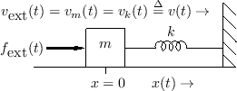
Figure 7.8 shows the electrical equivalent circuit corresponding to Fig.7.7.
 |
 |
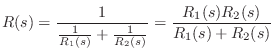
Parallel Combination of One-Ports
Figure Fig.7.10 shows the parallel combination of two one-ports.
![\includegraphics[scale=0.9]{eps/lparallel}](http://www.dsprelated.com/josimages_new/pasp/img1611.png) |
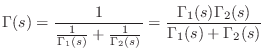
Admittances add in parallel, so the combined admittance is
![]() , and the impedance is
, and the impedance is
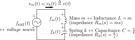
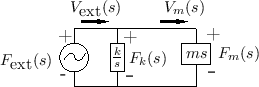
Spring-Mass System
When two physical elements are driven by a common force (yet
have independent velocities, as we'll soon see is quite possible),
they are formally in parallel. An example is a mass connected
to a spring in which the driving force is applied to one end of the
spring, and the mass is attached to the other end, as shown in
Fig.7.11. The compression force on the spring
is equal at all times to the rightward force on the mass. However,
the spring compression velocity ![]() does not always equal the
mass velocity
does not always equal the
mass velocity ![]() . We do have that the sum of the mass velocity
and spring compression velocity gives the velocity of the driving point,
i.e.,
. We do have that the sum of the mass velocity
and spring compression velocity gives the velocity of the driving point,
i.e.,
![]() . Thus, in a parallel connection, forces
are equal and velocities sum.
. Thus, in a parallel connection, forces
are equal and velocities sum.
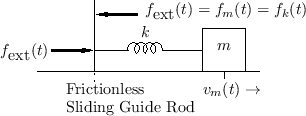
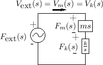
Figure 7.12 shows the electrical equivalent circuit corresponding to Fig.7.11.
 |
Mechanical Impedance Analysis
Impedance analysis is commonly used to analyze electrical circuits [110]. By means of equivalent circuits, we can use the same analysis methods for mechanical systems.
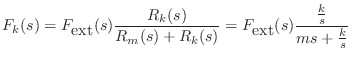
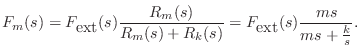
For example, referring to Fig.7.9, the Laplace transform of
the force on the spring ![]() is given by the so-called voltage
divider relation:8.2
is given by the so-called voltage
divider relation:8.2
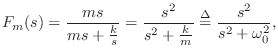
As a simple application, let's find the motion of the mass ![]() , after
time zero, given that the input force is an impulse at time 0:
, after
time zero, given that the input force is an impulse at time 0:
![\begin{eqnarray*}
V_m(s) &=& \frac{F_m(s)}{ms} \;=\; \frac{1}{m} \cdot \frac{s}{...
...}\right]\\ [5pt]
&\leftrightarrow& \frac{1}{m} \cos(\omega_0 t).
\end{eqnarray*}](http://www.dsprelated.com/josimages_new/pasp/img1626.png)
Thus, the impulse response of the mass oscillates sinusoidally with
radian frequency
![]() , and amplitude
, and amplitude ![]() . The
velocity starts out maximum at time
. The
velocity starts out maximum at time ![]() , which makes physical sense.
Also, the momentum transferred to the mass at time 0 is
, which makes physical sense.
Also, the momentum transferred to the mass at time 0 is
![]() ;
this is also expected physically because the time-integral of the applied
force is 1 (the area under any impulse
;
this is also expected physically because the time-integral of the applied
force is 1 (the area under any impulse ![]() is 1).
is 1).
General One-Ports
An arbitrary interconnection of ![]() impedances and admittances, with input
and output force and/or velocities defined, results in a one-port with
admittance expressible as
impedances and admittances, with input
and output force and/or velocities defined, results in a one-port with
admittance expressible as
Passive One-Ports
It is well known that the impedance of every passive one-port is positive real (see §C.11.2). The reciprocal of a positive real function is positive real, so every passive impedance corresponds also to a passive admittance.
A complex-valued function of a complex variable ![]() is said to be
positive real (PR) if
is said to be
positive real (PR) if
- 1)
 is real whenever
  is real
- 2)
-
 whenever
 .
.
A particularly important property of positive real
functions is that the phase is bounded between plus and minus ![]() degrees, i.e.,
degrees, i.e.,
![\includegraphics[width=\twidth]{eps/interlace}](http://www.dsprelated.com/josimages_new/pasp/img1637.png) |
Referring to Fig.7.14, consider the graphical method for
computing phase response of a reactance from the pole zero diagram
[449].8.4Each zero on the positive ![]() axis contributes a net 90 degrees
of phase at frequencies above the zero. As frequency crosses the zero
going up, there is a switch from
axis contributes a net 90 degrees
of phase at frequencies above the zero. As frequency crosses the zero
going up, there is a switch from ![]() to
to ![]() degrees. For each
pole, the phase contribution switches from
degrees. For each
pole, the phase contribution switches from ![]() to
to ![]() degrees as
it is passed going up in frequency. In order to keep phase in
degrees as
it is passed going up in frequency. In order to keep phase in
![]() , it is clear that the poles and zeros must strictly
alternate. Moreover, all poles and zeros must be simple, since a
multiple poles or zero would swing the phase by more than
, it is clear that the poles and zeros must strictly
alternate. Moreover, all poles and zeros must be simple, since a
multiple poles or zero would swing the phase by more than ![]() degrees, and the reactance could not be positive real.
degrees, and the reactance could not be positive real.
The positive real property is fundamental to passive immittances and comes up often in the study of measured resonant systems. A practical modeling example (passive digital modeling of a guitar bridge) is discussed in §9.2.1.
Digitization of Lumped Models
Since lumped models are described by differential equations, they are digitized (brought into the digital-signal domain) by converting them to corresponding finite-difference equations (or simply ``difference equations''). General aspects of finite difference schemes are discussed in Appendix D. This chapter introduces a couple of elementary methods in common use:
Note that digitization by the bilinear transform is closely related to the Wave Digital Filter (WDF) method introduced in Appendix F. Section 9.3.1 discusses a bilinearly transformed mass colliding with a digital waveguide string (an idealized struck-string example).
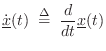
Finite Difference Approximation
A finite difference approximation (FDA) approximates derivatives with finite differences, i.e.,
![$\displaystyle \frac{d}{dt} x(t) \isdefs \lim_{\delta\to 0} \frac{x(t) - x(t-\delta)}{\delta} \;\approx\; \frac{x(n T)-x[(n-1)T]}{T} \protect$](http://www.dsprelated.com/josimages_new/pasp/img1643.png)
for sufficiently small
Equation (7.2) is also known as the backward difference approximation of differentiation.
See §C.2.1 for a discussion of using the FDA to model ideal vibrating strings.
FDA in the Frequency Domain
Viewing Eq.![]() (7.2) in the frequency domain, the ideal
differentiator transfer-function is
(7.2) in the frequency domain, the ideal
differentiator transfer-function is ![]() , which can be viewed as
the Laplace transform of the operator
, which can be viewed as
the Laplace transform of the operator ![]() (left-hand side of
Eq.
(left-hand side of
Eq.![]() (7.2)). Moving to the right-hand side, the z transform of the
first-order difference operator is
(7.2)). Moving to the right-hand side, the z transform of the
first-order difference operator is
![]() . Thus, in the
frequency domain, the finite-difference approximation may be performed
by making the substitution
. Thus, in the
frequency domain, the finite-difference approximation may be performed
by making the substitution
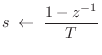
in any continuous-time transfer function (Laplace transform of an integro-differential operator) to obtain a discrete-time transfer function (z transform of a finite-difference operator).
The inverse of substitution Eq.![]() (7.3) is
(7.3) is
As discussed in §8.3.1, the FDA is a special case of the
matched ![]() transformation applied to the point
transformation applied to the point ![]() .
.
Note that the FDA does not alias, since the conformal mapping
![]() is one to one. However, it does warp the poles and zeros in a
way which may not be desirable, as discussed further on p.
is one to one. However, it does warp the poles and zeros in a
way which may not be desirable, as discussed further on p. ![]() below.
below.
Delay Operator Notation
It is convenient to think of the FDA in terms of time-domain
difference operators using a delay operator notation. The
delay operator ![]() is defined by
is defined by
The obvious definition for the second derivative is

However, a better definition is the centered finite difference
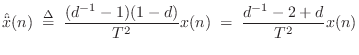
where
Bilinear Transformation
The bilinear transform is defined by the substitution
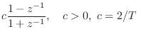 (typically)
where
It can be seen that analog dc (![]() ) maps to digital dc (
) maps to digital dc (![]() ) and
the highest analog frequency (
) and
the highest analog frequency (![]() ) maps to the highest digital
frequency (
) maps to the highest digital
frequency (![]() ). It is easy to show that the entire
). It is easy to show that the entire ![]() axis
in the
axis
in the ![]() plane (where
plane (where
![]() ) is mapped exactly
once around the unit circle in the
) is mapped exactly
once around the unit circle in the ![]() plane (rather than
summing around it infinitely many times, or ``aliasing'' as it does in
ordinary sampling). With
plane (rather than
summing around it infinitely many times, or ``aliasing'' as it does in
ordinary sampling). With ![]() real and positive, the left-half
real and positive, the left-half ![]() plane maps to the interior of the unit circle, and the right-half
plane maps to the interior of the unit circle, and the right-half ![]() plane maps outside the unit circle. This means stability is
preserved when mapping a continuous-time transfer function to
discrete time.
plane maps outside the unit circle. This means stability is
preserved when mapping a continuous-time transfer function to
discrete time.
Another valuable property of the bilinear transform is that
order is preserved. That is, an ![]() th-order
th-order ![]() -plane transfer
function carries over to an
-plane transfer
function carries over to an ![]() th-order
th-order ![]() -plane transfer function.
(Order in both cases equals the maximum of the degrees of the
numerator and denominator polynomials [449]).8.6
-plane transfer function.
(Order in both cases equals the maximum of the degrees of the
numerator and denominator polynomials [449]).8.6
The constant ![]() provides one remaining degree of freedom which can be used
to map any particular finite frequency from the
provides one remaining degree of freedom which can be used
to map any particular finite frequency from the ![]() axis in the
axis in the ![]() plane to a particular desired location on the unit circle
plane to a particular desired location on the unit circle
![]() in the
in the ![]() plane. All other frequencies will be warped. In
particular, approaching half the sampling rate, the frequency axis
compresses more and more. Note that at most one resonant frequency can be
preserved under the bilinear transformation of a mass-spring-dashpot
system. On the other hand, filters having a single transition frequency,
such as lowpass or highpass filters, map beautifully under the bilinear
transform; one simply uses
plane. All other frequencies will be warped. In
particular, approaching half the sampling rate, the frequency axis
compresses more and more. Note that at most one resonant frequency can be
preserved under the bilinear transformation of a mass-spring-dashpot
system. On the other hand, filters having a single transition frequency,
such as lowpass or highpass filters, map beautifully under the bilinear
transform; one simply uses ![]() to map the cut-off frequency where it
belongs, and the response looks great. In particular, ``equal ripple'' is
preserved for optimal filters of the elliptic and Chebyshev types because
the values taken on by the frequency response are identical in both cases;
only the frequency axis is warped.
to map the cut-off frequency where it
belongs, and the response looks great. In particular, ``equal ripple'' is
preserved for optimal filters of the elliptic and Chebyshev types because
the values taken on by the frequency response are identical in both cases;
only the frequency axis is warped.
The bilinear transform is often used to design digital filters from analog prototype filters [343]. An on-line introduction is given in [449].
Finite Difference Approximation vs. Bilinear Transform
Recall that the Finite Difference Approximation (FDA) defines the
elementary differentiator by
![]() (ignoring the
scale factor
(ignoring the
scale factor ![]() for now), and this approximates the ideal transfer
function
for now), and this approximates the ideal transfer
function ![]() by
by
![]() . The bilinear transform
calls instead for the transfer function
. The bilinear transform
calls instead for the transfer function
![]() (again
dropping the scale factor) which introduces a pole at
(again
dropping the scale factor) which introduces a pole at ![]() and gives
us the recursion
and gives
us the recursion
![]() .
Note that this new pole is right on the unit circle and is therefore
undamped. Any signal energy at half the sampling rate will circulate
forever in the recursion, and due to round-off error, it will tend to
grow. This is therefore a potentially problematic revision of the
differentiator. To get something more practical, we need to specify
that the filter frequency response approximate
.
Note that this new pole is right on the unit circle and is therefore
undamped. Any signal energy at half the sampling rate will circulate
forever in the recursion, and due to round-off error, it will tend to
grow. This is therefore a potentially problematic revision of the
differentiator. To get something more practical, we need to specify
that the filter frequency response approximate
![]() over a
finite range of frequencies
over a
finite range of frequencies
![]() , where
, where
![]() , above which we allow the response to ``roll off''
to zero. This is how we pose the differentiator problem in terms of
general purpose filter design (see §8.6) [362].
, above which we allow the response to ``roll off''
to zero. This is how we pose the differentiator problem in terms of
general purpose filter design (see §8.6) [362].
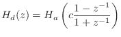
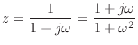
To understand the properties of the finite difference approximation in the
frequency domain, we may look at the properties of its ![]() -plane
to
-plane
to ![]() -plane mapping
-plane mapping

Setting ![]() to 1 for simplicity and solving the FDA mapping for z gives
to 1 for simplicity and solving the FDA mapping for z gives
![\includegraphics[width=3in]{eps/lfdacirc}](http://www.dsprelated.com/josimages_new/pasp/img1678.png)
Under the FDA, analog and digital frequency axes coincide well enough at
very low frequencies (high sampling rates), but at high frequencies
relative to the sampling rate, artificial damping is introduced as
the image of the ![]() axis diverges away from the unit circle.
axis diverges away from the unit circle.
While the bilinear transform ``warps'' the frequency axis, we can say the FDA ``doubly warps'' the frequency axis: It has a progressive, compressive warping in the direction of increasing frequency, like the bilinear transform, but unlike the bilinear transform, it also warps normal to the frequency axis.
Consider a point traversing the upper half of the unit circle in the z
plane, starting at ![]() and ending at
and ending at ![]() . At dc, the FDA is
perfect, but as we proceed out along the unit circle, we diverge from the
. At dc, the FDA is
perfect, but as we proceed out along the unit circle, we diverge from the
![]() axis image and carve an arc somewhere out in the image of the
right-half
axis image and carve an arc somewhere out in the image of the
right-half ![]() plane. This has the effect of introducing an artificial
damping.
plane. This has the effect of introducing an artificial
damping.
Consider, for example, an undamped mass-spring system. There will be a
complex conjugate pair of poles on the ![]() axis in the
axis in the ![]() plane. After
the FDA, those poles will be inside the unit circle, and therefore damped
in the digital counterpart. The higher the resonance frequency, the larger
the damping. It is even possible for unstable
plane. After
the FDA, those poles will be inside the unit circle, and therefore damped
in the digital counterpart. The higher the resonance frequency, the larger
the damping. It is even possible for unstable ![]() -plane poles to be mapped
to stable
-plane poles to be mapped
to stable ![]() -plane poles.
-plane poles.
In summary, both the bilinear transform and the FDA preserve order,
stability, and positive realness. They are both free of aliasing, high
frequencies are compressively warped, and both become ideal at dc, or as
![]() approaches
approaches ![]() . However, at frequencies significantly above
zero relative to the sampling rate, only the FDA introduces artificial
damping. The bilinear transform maps the continuous-time frequency axis in
the
. However, at frequencies significantly above
zero relative to the sampling rate, only the FDA introduces artificial
damping. The bilinear transform maps the continuous-time frequency axis in
the ![]() (the
(the ![]() axis) plane precisely to the discrete-time frequency
axis in the
axis) plane precisely to the discrete-time frequency
axis in the ![]() plane (the unit circle).
plane (the unit circle).
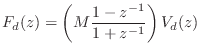
Application of the Bilinear Transform
The impedance of a mass in the frequency domain is
![\begin{eqnarray*}
(1+z^{-1})F_d(z) &=& M (1-z^{-1}) V_d(z) \\
\;\longleftrighta...
...
\,\,\Rightarrow\,\,f_d(n) &=& M[v_d(n) - v_d(n-1)] - f_d(n-1).
\end{eqnarray*}](http://www.dsprelated.com/josimages_new/pasp/img1686.png)
This difference equation is diagrammed in Fig. 7.16. We recognize this recursive digital filter as the direct form I structure. The direct-form II structure is obtained by commuting the feedforward and feedback portions and noting that the two delay elements contain the same value and can therefore be shared [449]. The two other major filter-section forms are obtained by transposing the two direct forms by exchanging the input and output, and reversing all arrows. (This is a special case of Mason's Gain Formula which works for the single-input, single-output case.) When a filter structure is transposed, its summers become branching nodes and vice versa. Further discussion of the four basic filter section forms can be found in [333].
![\includegraphics[width=4in]{eps/lmassFilterDF1}](http://www.dsprelated.com/josimages_new/pasp/img1687.png) |
Practical Considerations
While the digital mass simulator has the desirable properties of the bilinear transform,
it is also not perfect from a practical point of view:
(1) There is a pole at half the sampling rate (![]() ).
(2) There is a delay-free path from input to output.
).
(2) There is a delay-free path from input to output.
The first problem can easily be circumvented by introducing a loss factor ![]() ,
moving the pole from
,
moving the pole from ![]() to
to ![]() , where
, where ![]() and
and ![]() . This
is sometimes called the ``leaky integrator''.
. This
is sometimes called the ``leaky integrator''.
The second problem arises when making loops of elements (e.g., a mass-spring chain which forms a loop). Since the individual elements have no delay from input to output, a loop of elements is not computable using standard signal processing methods. The solution proposed by Alfred Fettweis is known as ``wave digital filters,'' a topic taken up in §F.1.
Limitations of Lumped Element Digitization
Model discretization by the FDA (§7.3.1) and bilinear transform (§7.3.2) methods are order preserving. As a result, they suffer from significant approximation error, especially at high frequencies relative to half the sampling rate. By allowing a larger order in the digital model, we may obtain arbitrarily accurate transfer-function models of LTI subsystems, as discussed in Chapter 8. Of course, in higher-order approximations, the state variables of the simulation no longer have a direct physical intepretation, and this can have implications, particularly when trying to extend to the nonlinear case. The benefits of a physical interpretation should not be given up lightly. For example, one may consider oversampling in place of going to higher-order element approximations.
More General Finite-Difference Methods
The FDA and bilinear transform of the previous sections can be viewed
as first-order conformal maps from the analog ![]() plane to the digital
plane to the digital
![]() plane. These maps are one-to-one and therefore non-aliasing. The
FDA performs well at low frequencies relative to the sampling rate,
but it introduces artificial damping at high frequencies. The
bilinear transform preserves the frequency axis exactly, but over a
warped frequency scale. Being first order, both maps preserve the
number of poles and zeros in the model.
plane. These maps are one-to-one and therefore non-aliasing. The
FDA performs well at low frequencies relative to the sampling rate,
but it introduces artificial damping at high frequencies. The
bilinear transform preserves the frequency axis exactly, but over a
warped frequency scale. Being first order, both maps preserve the
number of poles and zeros in the model.
We may only think in terms of mapping the ![]() plane to the
plane to the ![]() plane
for linear, time-invariant systems. This is because Laplace
transform analysis is not defined for nonlinear and/or time-varying
differential equations (no
plane
for linear, time-invariant systems. This is because Laplace
transform analysis is not defined for nonlinear and/or time-varying
differential equations (no ![]() plane). Therefore, such systems are
instead digitized by some form of numerical integration to
produce solutions that are ideally sampled versions of the
continuous-time solutions. It is often necessary to work at sampling
rates much higher than the desired audio sampling rate, due to the
bandwidth-expanding effects of nonlinear elements in the
continuous-time system.
plane). Therefore, such systems are
instead digitized by some form of numerical integration to
produce solutions that are ideally sampled versions of the
continuous-time solutions. It is often necessary to work at sampling
rates much higher than the desired audio sampling rate, due to the
bandwidth-expanding effects of nonlinear elements in the
continuous-time system.
A tutorial review of numerical solutions of Ordinary Differential Equations (ODE), including nonlinear systems, with examples in the realm of audio effects (such as a diode clipper), is given in [555]. Finite difference schemes specifically designed for nonlinear discrete-time simulation, such as the energy-preserving ``Kirchoff-Carrier nonlinear string model'' and ``von Karman nonlinear plate model'', are discussed in [53].
The remaining sections here summarize a few of the more elementary techniques discussed in [555].
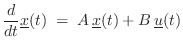
General Nonlinear ODE
In state-space form (§1.3.7) [449],8.7a general class of ![]() th-order Ordinary Differential Equations (ODE),
can be written as
th-order Ordinary Differential Equations (ODE),
can be written as
where
In the linear, time-invariant (LTI) case, Eq.![]() (7.8) can be
expressed in the usual state-space form for LTI continuous-time
systems:
(7.8) can be
expressed in the usual state-space form for LTI continuous-time
systems:
In this case, standard methods for converting a filter from continuous to discrete time may be used, such as the FDA (§7.3.1) and bilinear transform (§7.3.2).8.8
Forward Euler Method
The finite-difference approximation (Eq.![]() (7.2)) with the
derivative evaluated at time
(7.2)) with the
derivative evaluated at time ![]() yields the forward Euler
method of numerical integration:
yields the forward Euler
method of numerical integration:
where
Because each iteration of the forward Euler method depends only on
past quantities, it is termed an explicit method. In the LTI
case, an explicit method corresponds to a causal digital filter
[449]. Methods that depend on current and/or future
solution samples (i.e.,
![]() for
for ![]() ) are
called implicit methods. When a nonlinear
numerical-integration method is implicit, each step forward in time
typically uses some number of iterations of Newton's Method (see
§7.4.5 below).
) are
called implicit methods. When a nonlinear
numerical-integration method is implicit, each step forward in time
typically uses some number of iterations of Newton's Method (see
§7.4.5 below).
Backward Euler Method
An example of an implicit method is the backward Euler method:
Because the derivative is now evaluated at time
Trapezoidal Rule
The trapezoidal rule is defined by
Thus, the trapezoidal rule is driven by the average of the derivative estimates at times
The trapezoidal rule gets its name from the fact that it approximates
an integral by summing the areas of trapezoids. This can be seen by writing
Eq.![]() (7.12) as
(7.12) as
An interesting fact about the trapezoidal rule is that it is
equivalent to the bilinear transform in the linear,
time-invariant case. Carrying Eq.![]() (7.12) to the frequency domain
gives
(7.12) to the frequency domain
gives
![\begin{eqnarray*}
X(z) &=& z^{-1}X(z) + T\, \frac{s X(z) + z^{-1}s X(z)]}{2}\\
...
...gleftrightarrow\quad s &=& \frac{2}{T}\frac{1-z^{-1}}{1+z^{-1}}.
\end{eqnarray*}](http://www.dsprelated.com/josimages_new/pasp/img1709.png)
Newton's Method of Nonlinear Minimization
Newton's method [162],[166, p. 143] finds the minimum of a nonlinear (scalar) function of several variables by locally approximating the function by a quadratic surface, and then stepping to the bottom of that ``bowl'', which generally requires a matrix inversion. Newton's method therefore requires the function to be ``close to quadratic'', and its effectiveness is directly tied to the accuracy of that assumption. For smooth functions, Newton's method gives very rapid quadratic convergence in the last stages of iteration. Quadratic convergence implies, for example, that the number of significant digits in the minimizer approximately doubles each iteration.
Newton's method may be derived as follows: Suppose we wish to minimize
the real, positive function
![]() with respect to
with respect to
![]() . The
vector Taylor expansion [546] of
. The
vector Taylor expansion [546] of
![]() about
about
![]() gives
gives
Applying Eq.
where
When the
![]() is any quadratic form in
is any quadratic form in
![]() , then
, then
![]() , and
Newton's method produces
, and
Newton's method produces
![]() in one iteration; that is,
in one iteration; that is,
![]() for every
for every
![]() .
.
Semi-Implicit Methods
A semi-implicit method for numerical integration is based on an
implicit method by using only one iteration of Newton's method
[354,555]. This effectively converts the implicit
method into a corresponding explicit method. Best results are
obtained for highly oversampled systems (i.e., ![]() is larger
than typical audio sampling rates).
is larger
than typical audio sampling rates).
Semi-Implicit Backward Euler
The semi-implicit backward Euler method is defined by [555]
![$\displaystyle \underline{\hat{x}}(n) \isdefs \underline{\hat{x}}(n-1) + T\, \frac{f[n,\underline{\hat{x}}(n-1)]}{1-T\,\ddot{\underline{\hat{x}}}(n-1)} \protect$](http://www.dsprelated.com/josimages_new/pasp/img1725.png)
where
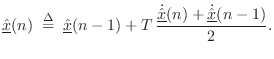
Semi-Implicit Trapezoidal Rule
The semi-implicit trapezoidal rule method is given by [555]
![$\displaystyle \underline{\hat{x}}(n) \isdefs \underline{\hat{x}}(n-1) + \frac{T...
...rline{\hat{x}}(n-1)]}{1-\frac{T}{2}\,\ddot{\underline{\hat{x}}}(n-1)}. \protect$](http://www.dsprelated.com/josimages_new/pasp/img1728.png)
Summary
We have looked at a number of methods for solving nonlinear ordinary differential equations, including explicit, implicit, and semi-implicit numerical integration methods. Specific methods included the explicit forward Euler (similar to the finite difference approximation of §7.3.1), backward Euler (implicit), trapezoidal rule (implicit, and equivalent to the bilinear transform of §7.3.2 in the LTI case), and semi-implicit variants of the backward Euler and trapezoidal methods.
As demonstrated and discussed further in [555], implicit methods are generally more accurate than explicit methods for nonlinear systems, with semi-implicit methods (§7.4.6) typically falling somewhere in between. Semi-implicit methods therefore provide a source of improved explicit methods. See [555] and the references therein for a discussion of accuracy and stability of such schemes, as well as applied examples.
Further Reading in Nonlinear Methods
Other well known numerical integration methods for ODEs include second-order backward difference formulas (commonly used in circuit simulation [555]), the fourth-order Runge-Kutta method [99], and their various explicit, implicit, and semi-implicit variations. See [555] for further discussion of these and related finite-difference schemes, and for application examples in the virtual analog area (digitization of musically useful analog circuits). Specific digitization problems addressed in [555] include electric-guitar distortion devices [553,556], the classic ``tone stack'' [552] (an often-used bass, midrange, and treble control circuit in guitar amplifiers), the Moog VCF, and other electronic components of amplifiers and effects. Also discussed in [555] is the ``K Method'' for nonlinear system digitization, with comparison to nonlinear wave digital filters (see Appendix F for an introduction to linear wave digital filters).
The topic of real-time finite difference schemes for virtual analog systems remains a lively research topic [554,338,293,84,264,364,397].
For Partial Differential Equations (PDEs), in which spatial derivatives are mixed with time derivatives, the finite-difference approach remains fundamental. An introduction and summary for the LTI case appear in Appendix D. See [53] for a detailed development of finite difference schemes for solving PDEs, both linear and nonlinear, applied to digital sound synthesis. Physical systems considered in [53] include bars, stiff strings, bow coupling, hammers and mallets, coupled strings and bars, nonlinear strings and plates, and acoustic tubes (voice, wind instruments). In addition to numerous finite-difference schemes, there are chapters on finite-element methods and spectral methods.
Summary of Lumped Modeling
In this chapter, we looked at the fundamentals of lumped modeling elements such as masses, springs, and dashpots. The important concept of driving-point impedance was defined and discussed, and electrical equivalent circuits were developed, along with associated elementary (circuit) network theory. Finally, we looked at basic ways of digitizing lumped elements and more complex ODEs and PDEs, including a first glance at some nonlinear methods.
Practical examples of lumped models begin in §9.3.1. In particular, piano-like models require a ``hammer'' to strike the string, and §9.3.1 explicates the simplest case of an ideal point-mass striking an ideal vibrating string. In that model, when the mass is in contact with the string, it creates a scattering junction on the string having reflection and transmission coefficients that are first-order filters. These filters are then digitized via the bilinear transform. The ideal string itself is of course modeled as a digital waveguide. A detailed development of wave scattering at impedance-discontinuities is presented for digital waveguide models in §C.8, and for wave digital filters in Appendix F.
Next Section:
Transfer Function Models
Previous Section:
Digital Waveguide Models


