Root-Power Waves
It is sometimes helpful to normalize the wave variables so that
signal power is uniformly distributed numerically. This can be especially
helpful in fixed-point implementations.
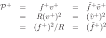
From (C.49), it is clear that power normalization is given by
 |
(C.53) |
where we have dropped the common time argument `

' for simplicity.
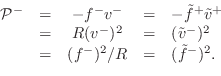
As a result, we obtain
and
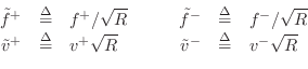
The normalized
wave variables

and

behave physically like
force and
velocity waves, respectively, but they are scaled such that
either can be squared to obtain instantaneous
signal power.
Waveguide
networks built using normalized waves have many desirable properties
[
174,
172,
432]. One is the obvious numerical
advantage of uniformly distributing signal power across available
dynamic
range in
fixed-point implementations. Another is that only in the
normalized case can the
wave impedances be made
time varying without modulating
signal power. In other words, use of normalized waves eliminates
``parametric amplification'' effects; signal power is decoupled from
parameter changes.
Next Section: Total Energy in a Rigidly Terminated StringPrevious Section: Energy Density Waves