Tonehole Modeling

Toneholes in woodwind instruments are essentially cylindrical holes in the bore. One modeling approach would be to treat the tonehole as a small waveguide which connects to the main bore via one port on a three-port junction. However, since the tonehole length is small compared with the distance sound travels in one sampling instant ( in, e.g.), it is more straightforward to treat the tonehole as a lumped load along the bore, and most modeling efforts have taken this approach.

The musical acoustics literature contains experimentally verified models of tone-hole acoustics, such as by Keefe [238]. Keefe's tonehole model is formulated as a ``transmission matrix'' description, which we may convert to a traveling-wave formulation by a simple linear transformation (described in §9.5.4 below) [465]. For typical fingerings, the first few open tone holes jointly provide a bore termination [38]. Either the individual tone holes can be modeled as (interpolated) scattering junctions, or the whole ensemble of terminating tone holes can be modeled in aggregate using a single reflection and transmission filter, like the bell model. Since the tone hole diameters are small compared with most audio frequency wavelengths, the reflection and transmission coefficients can be implemented to a reasonable approximation as constants, as opposed to cross-over filters as in the bell. Taking into account the inertance of the air mass in the tone hole, the tone hole can be modeled as a two-port loaded junction having load impedance equal to the air-mass inertance [143,509]. At a higher level of accuracy, adapting transmission-matrix parameters from the existing musical acoustics literature leads to first-order reflection and transmission filters [238,406,403,404,465]. The individual tone-hole models can be simple lossy two-port junctions, modeling only the internal bore loss characteristics, or three-port junctions, modeling also the transmission characteristics to the outside air. Another approach to modeling toneholes is the ``wave digital'' model [527] (see §F.1 for a tutorial introduction to this approach). The subject of tone-hole modeling is elaborated further in [406,502]. For simplest practical implementation, the bell model can be used unchanged for all tunings, as if the bore were being cut to a new length for each note and the same bell were attached. However, for best results in dynamic performance, the tonehole model should additionally include an explicit valve model for physically accurate behavior when slowly opening or closing the tonehole [405].

The Clarinet Tonehole as a Two-Port Junction

The clarinet tonehole model developed by Keefe [240] is parametrized in terms of series and shunt resistance and reactance, as shown in Fig. 9.43. The transmission matrix description of this two-port is given by the product of the transmission matrices for the series impedance , shunt impedance , and series impedance , respectively:

where all quantities are written in the frequency domain, and the impedance parameters are given by

where is the wave impedance of the tonehole entrance, i.e., that of an acoustic tube of cross-sectional area ( is air density and is sound speed as usual), is the tonehole radius, is the wavenumber (radian spatial frequency), is the open-tonehole effective length (which is slightly greater than its physical length due to the formation of a small air-piston inside the open tonehole), is the ``specific resistance'' of the open tonehole due to air viscosity in and radiation from the hole, is the closed-tonehole height, defined such that its product times the cross-sectional area of the tonehole exactly equals the geometric volume of the closed tonehole. Finally, and are the equivalent series lengths of the open and closed tonehole, respectively, and are given by

where is the radius of the main bore. The closed-tonehole height can be estimated as [240]

where is the physical tonehole chimney height at its center.

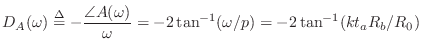
Note that the specific resistance of the open tonehole, , is the only real impedance and therefore the only source of wave energy loss at the tonehole. It is given by [240]

where is the radius of curvature of the tonehole, is the viscous boundary layer thickness which expressible in terms of the shear viscosity of air as

and is the real part of the propagation wavenumber (or minus the imaginary part of complex spatial frequency ). In [239], for the large-tube limit (i.e., when the tube radius is large compared with the viscous boundary layer), is given by

where is the adiabatic gas constant for air [318], is the thermal conductivity of air, and is the specific heat of air at constant pressure. In [239], the following values are given for air at Kelvin ( C), and valid within degrees of that temperature:

where

can be interpreted as times the ratio of the tonehole radius to the viscous boundary layer thickness [239]. The constant is referred to as the Prandtl number, and is the shear viscosity coefficient [239]. In [71], it is noted that is greater than under practical conditions in musical acoustics, and so it is therefore sufficient to keep only the first and second-order terms in the expression above for .

The open-hole effective length , assuming no pad above the hole, is given in [240] as

See [240] for the case in which a pad lies above the open hole. In [405], a unified tonehole model is given which supports continuous opening and closing of the tonehole.

For implementation in a digital waveguide model, the lumped parameters above must be converted to scattering parameters. Such formulations of toneholes have appeared in the literature: Vesa Välimäki [509,502] developed tonehole models based on a ``three-port'' digital waveguide junction loaded by an inertance, as described in Fletcher and Rossing [143], and also extended his results to the case of interpolated digital waveguides. It should be noted in this context, however, that in the terminology of Appendix C, Välimäki's tonehole representation is a loaded 2-port junction rather than a three-port junction. (A load can be considered formally equivalent to a ``waveguide'' having wave impedance given by the load impedance.) Scavone and Smith [402] developed digital waveguide tonehole models based on the more rigorous ``symmetric T'' acoustic model of Keefe [240], using general purpose digital filter design techniques to obtain rational approximations to the ideal tonehole frequency response. A detailed treatment appears in Scavone's CCRMA Ph.D. thesis [406]. This section, adapted from [465], considers an exact translation of the Keefe tonehole model, obtaining two one-filter implementations: the ``shared reflectance'' and ``shared transmittance'' forms. These forms are shown to be stable without introducing an approximation which neglects the series inertance terms in the tonehole model.

By substituting in (9.53) to convert spatial frequency to temporal frequency, and by substituting

for , into (9.51) to convert physical variables to wave variables, ( is the bore wave impedance), we may solve for the outgoing waves in terms of the incoming waves . Mathematica code for obtaining the general conversion formula from lumped parameters to scattering parameters is as follows:

        Clear["t*", "p*", "u*", "r*"]
        transmissionMatrix = {{t11, t12}, {t21, t22}};
        leftPort = {{p2p+p2m}, {(p2p-p2m)/r2}};
        rightPort = {{p1p+p1m}, {(p1p-p1m)/r1}};
        Format[t11, TeXForm] := "{T_{11}}"
        Format[p1p, TeXForm] := "{P_1^+}"
        ... (etc. for all variables) ...
        TeXForm[Simplify[Solve[leftPort ==
               transmissionMatrix . rightPort, {p1m, p2p}]]]

The above code produces the following formulas:

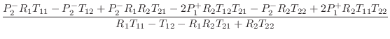
Substituting relevant values for Keefe's tonehole model, we obtain, in matrix notation,

We thus obtain the scattering formulation depicted in Fig. 9.44, where

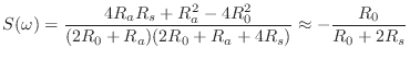
is the reflectance of the tonehole (the same from either direction), and

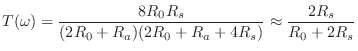
is the transmittance of the tonehole (also the same from either direction). The notation ``'' for reflectance is chosen because every reflectance is a Schur function (stable and not exceeding unit magnitude on the unit circle in the plane) [428, p. 221].

The approximate forms in (9.57) and (9.58) are obtained by neglecting the negative series inertance which serves to adjust the effective length of the bore, and which therefore can be implemented elsewhere in the interpolated delay-line calculation as discussed further below. The open and closed tonehole cases are obtained by substituting and , respectively, from (9.53).

In a manner analogous to converting the four-multiply Kelly-Lochbaum (KL) scattering junction [245] into a one-multiply form (cf. (C.60) and (C.62) on page ), we may pursue a ``one-filter'' form of the waveguide tonehole model. However, the series inertance gives some initial trouble, since

instead of zero as in the KL junction. In the scattering formulas (C.100) and (C.101) on page  for the general loaded waveguide junction, the reflectance seen on any branch is always the transmittance from that branch to any other branch minus . I.e., if denotes the transmittance from branch to all other branches meeting at the junction, then is the reflectance seen on branch . Substituting

into the basic scattering relations (9.56), and factoring out , we obtain, in the frequency domain,

and, similarly,

The resulting tonehole implementation is shown in Fig. 9.45. We call this the ``shared reflectance'' form of the tonehole junction.

In the same way, an alternate form is obtained from the substitution

which yields the ``shared transmittance'' form:

shown in Fig. 9.46.

Since , it can be neglected to first order, and , reducing both of the above forms to an approximate ``one-filter'' tonehole implementation.

Since is a pure negative reactance, we have

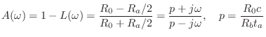
In this form, it is clear that is a first-order allpass filter with a single pole-zero pair near infinity. Unfortunately, the pole is in the right-half-plane and hence unstable. We cannot therefore implement it as shown in Fig. 9.45 or Fig. 9.46. Using elementary manipulations, the unstable allpasses in Figs. 9.45 and Fig. 9.46 can be moved to the configuration shown in Figs. 9.47 and 9.48, respectively. Note that is stable whenever is stable. The unstable allpasses now operate only on the two incoming wave variables, and they can be implemented implicitly by slightly reducing the (interpolated) delay-lines leading to the junction from either side. The tonehole then requires only one filter or .

We now see precisely how the negative series inertance provides a negative, frequency-dependent, length correction for the bore. From (9.63), the phase delay of can be computed as

Thus, the negative delay correction goes to zero with frequency , series tonehole length , tonehole impedance , or main bore admittance .

In practice, it is common to combine all delay corrections into a single ``tuning allpass filter'' for the whole bore [428,207]. Whenever the desired allpass delay goes negative, we simply add a sample of delay to the desired allpass phase-delay and subtract it from the nearest delay. In other words, negative delays have to be ``pulled out'' of the allpass and used to shorten an adjacent interpolated delay line. Such delay lines are normally available in practical modeling situations.

---

Tonehole Filter Design

The tone-hole reflectance and transmittance must be converted to discrete-time form for implementation in a digital waveguide model. Figure 9.49 plots the responses of second-order discrete-time filters designed to approximate the continuous-time magnitude and phase characteristics of the reflectances for closed and open toneholes, as carried out in [403,406]. These filter designs assumed a tonehole of radius mm, minimum tonehole height mm, tonehole radius of curvature mm, and air column radius mm. Since the measurements of Keefe do not extend to 5 kHz, the continuous-time responses in the figures are extrapolated above this limit. Correspondingly, the filter designs were weighted to produce best results below 5 kHz.

The closed-hole filter design was carried out using weighted equation-error minimization [428, p. 47], i.e., by minimizing , where is the weighting function, is the desired frequency response, denotes discrete-time radian frequency, and the designed filter response is . Note that both phase and magnitude are matched by equation-error minimization, and this error criterion is used extensively in the field of system identification [288] due to its ability to design optimal IIR filters via quadratic minimization. In the spirit of the well-known Steiglitz-McBride algorithm [287], equation-error minimization can be iterated, setting the weighting function at iteration to the inverse of the inherent weighting of the previous iteration, i.e., . However, for this study, the weighting was used only to increase accuracy at low frequencies relative to high frequencies. Weighted equation-error minimization is implemented in the matlab function invfreqz() (§8.6.4).

The open-hole discrete-time filter was designed using Kopec's method [297], [428, p. 46] in conjunction with weighted equation-error minimization. Kopec's method is based on linear prediction:

• Given a desired complex frequency response , compute an allpole model using linear prediction
• Compute the error spectrum .
• Compute an allpole model for by minimizing
  

Use of linear prediction is equivalent to minimizing the ratio error

This optimization criterion causes the filter to fit the upper spectral envelope of the desired frequency-response. Since the first step of Kopec's method captures the upper spectral envelope, the ``nulls'' and ``valleys'' are largely ``saved'' for the next step which computes zeros. When computing the zeros, the spectral ``dips'' become ``peaks,'' thereby receiving more weight under the ratio-error norm. Thus, in Kopec's method, the poles model the upper spectral envelope, while the zeros model the lower spectral envelope. To apply Kopec's method to the design of an open-tonehole filter, a one-pole model was first fit to the continuous-time response, Subsequently, the inverse error spectrum, was modeled with a two-pole digital filter, The discrete-time approximation to was then given by

The reasonably close match in both phase and magnitude by second-order filters indicates that there is in fact only one important tonehole resonance and/or anti-resonance within the audio band, and that the measured frequency responses can be modeled with very high audio accuracy using only second-order filters.

Figure 9.50 plots the reflection function calculated for a six-hole flute bore, as described in [240].

The upper plot was calculated using Keefe's frequency-domain transmission matrices, such that the reflection function was determined as the inverse Fourier transform of the corresponding reflection coefficient. This response is equivalent to that provided by [240], though scale factor discrepancies exist due to differences in open-end reflection models and lowpass filter responses. The lower plot was calculated from a digital waveguide model using two-port tonehole scattering junctions. Differences between the continuous- and discrete-time results are most apparent in early, high-frequency, closed-hole reflections. The continuous-time reflection function was low-pass filtered to remove time-domain aliasing effects incurred by the inverse Fourier transform operation and to better correspond with the plots of [240]. By trial and error, a lowpass filter with a cutoff frequency around 4 kHz was found to produce the best match to Keefe's results. The digital waveguide result was obtained at a sampling rate of 44.1 kHz and then lowpass filtered to a 10 kHz bandwidth, corresponding to that of [240]. Further lowpass filtering is inherent from the first-order Lagrangian, delay-line length interpolation technique used in this model [502]. Because such filtering is applied at different locations along the ``bore,'' a cumulative effect is difficult to accurately determine. The first tonehole reflection is affected by only two interpolation filters, while the second tonehole reflection is affected by four of these filtering operations. This effect is most responsible for the minor discrepancies apparent in the plots.

---

The Tonehole as a Two-Port Loaded Junction

It seems reasonable to expect that the tonehole should be representable as a load along a waveguide bore model, thus creating a loaded two-port junction with two identical bore ports on either side of the tonehole. From the relations for the loaded parallel junction (C.101), in the two-port case with , and considering pressure waves rather than force waves, we have

Thus, the loaded two-port junction can be implemented in ``one-filter form'' as shown in Fig. 9.48 with ( ) and

Comparing with (9.58), we see that the simplified Keefe tonehole model with the negative series inertance removed (), is equivalent to a loaded two-port waveguide junction with , i.e., the parallel load impedance is simply the shunt impedance in the tonehole model.

Each series impedance in the split-T model of Fig. 9.43 can be modeled as a series waveguide junction with a load of . To see this, set the transmission matrix parameters in (9.55) to the values , , and from (9.51) to get

where is the alpha parameter for a series loaded waveguide junction involving two impedance waveguides joined in series with each other and with a load impedance of , as can be seen from (C.99). To obtain exactly the loaded series scattering relations (C.100), we first switch to the more general convention in which the ``'' superscript denotes waves traveling into a junction of any number of waveguides. This exchanges ``'' with ``'' at port 2 to yield

Next we convert pressure to velocity using and to obtain

Finally, we toggle the reference direction of port 2 (the ``current'' arrow for on port 2 in Fig. 9.43) so that velocity is positive flowing into the junction on both ports (which is the convention used to derive (C.100) and which is typically followed in circuit theory). This amounts to negating , giving

where . This is then the canonical form (C.100).

---

Next Section:
Digital Waveguide Bowed-String
Previous Section:
Single-Reed Theory

Sign in