


Well Posed Initial-Value Problem
For a proper authoritative definition of ``well posed'' in the field of finite-difference schemes, see, e.g., [481]. The definition we will use here is less general in that it excludes amplitude growth from initial conditions which is faster than polynomial in time.
We will say that an initial-value problem is well posed if the linear system defined by the PDE, together with any bounded initial conditions is marginally stable.
As discussed in [449], a system is defined to be stable when its response to bounded initial conditions approaches zero as time goes to infinity. If the response fails to approach zero but does not exponentially grow over time (the lossless case), it is called marginally stable.
In the literature on finite-difference schemes, lossless systems are classified as stable [481]. However, in this book series, lossless systems are not considered stable, but only marginally stable.
When marginally stable systems are allowed, it is necessary to accommodate polynomial growth with respect to time. As is well known in linear systems theory, repeated poles can yield polynomial growth [449]. A very simple example is the ordinary differential equation (ODE)
When all poles of the system are strictly in the left-half of the
Laplace-transform ![]() plane, the system is stable, even when
the poles are repeated. This is because exponentials are faster than
polynomials, so that any amount of exponential decay will eventually
overtake polynomial growth and drag it to zero in the limit.
plane, the system is stable, even when
the poles are repeated. This is because exponentials are faster than
polynomials, so that any amount of exponential decay will eventually
overtake polynomial growth and drag it to zero in the limit.
Marginally stable systems arise often in computational physical
modeling. In particular, the ideal string is only marginally stable,
since it is lossless. Even a simple unaccelerated mass, sliding on a
frictionless surface, is described by a marginally stable PDE when the
position of the mass is used as a state variable (see
§7.1.2). Given any nonzero initial velocity, the position
of the mass approaches either ![]() or
or ![]() infinity, exactly as in the
infinity, exactly as in the
![]() example above. To avoid unbounded growth in practical
systems, it is often preferable to avoid the use of displacement as a
state variable. For ideal strings and freely sliding masses, force
and velocity are usually good choices.
example above. To avoid unbounded growth in practical
systems, it is often preferable to avoid the use of displacement as a
state variable. For ideal strings and freely sliding masses, force
and velocity are usually good choices.
It should perhaps be emphasized that the term ``well posed'' normally allows for more general energy growth at a rate which can be bounded over all initial conditions [481]. In this book, however, the ``marginally stable'' case (at most polynomial growth) is what we need. The reason is simply that we wish to excluded unstable PDEs as a modeling target. Note, however, that unstable systems can be used profitable over carefully limited time durations (see §9.7.2 for an example).
In the ideal vibrating string, energy is conserved. Therefore, it is a
marginally stable system. To show mathematically that the PDE
Eq.![]() (D.2) is marginally stable, we may show that
(D.2) is marginally stable, we may show that
Note that solutions on the ideal string are not bounded, since, for
example, an infinitely long string (non-terminated) can be initialized
with a constant positive velocity everywhere along its length. This
corresponds physically to a nonzero transverse momentum, which is
conserved. Therefore, the string will depart in the positive ![]() direction, with an average displacement that grows linearly with
direction, with an average displacement that grows linearly with ![]() .
.
The well-posedness of a class of damped PDEs used in string modeling is analyzed in §D.2.2.
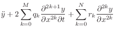
A Class of Well Posed Damped PDEs
A large class of well posed PDEs is given by [45]
Thus, to the ideal string wave equation Eq.
To show Eq.![]() (D.5) is well posed [45], we must
show that the roots of the characteristic polynomial equation
(§D.3) have negative real parts, i.e., that they correspond to
decaying exponentials instead of growing exponentials. To do this, we
may insert the general eigensolution
(D.5) is well posed [45], we must
show that the roots of the characteristic polynomial equation
(§D.3) have negative real parts, i.e., that they correspond to
decaying exponentials instead of growing exponentials. To do this, we
may insert the general eigensolution
Let's now set ![]() , where
, where
![]() is radian spatial
frequency (called the ``wavenumber'' in acoustics) and of course
is radian spatial
frequency (called the ``wavenumber'' in acoustics) and of course
![]() , thereby converting the implicit spatial Laplace
transform to a spatial Fourier transform. Since there are only even
powers of the spatial Laplace transform variable
, thereby converting the implicit spatial Laplace
transform to a spatial Fourier transform. Since there are only even
powers of the spatial Laplace transform variable ![]() , the polynomials
, the polynomials
![]() and
and ![]() are real. Therefore, the roots of the
characteristic polynomial equation (the natural frequencies of the
time response of the system), are given by
are real. Therefore, the roots of the
characteristic polynomial equation (the natural frequencies of the
time response of the system), are given by
Proof that the Third-Order Time Derivative is Ill Posed
For its tutorial value, let's also show that the PDE of Ruiz
[392] is ill posed, i.e., that at least one component of the
solution is a growing exponential. In this case, setting
![]() in Eq.
in Eq.![]() (C.28), which we restate as
(C.28), which we restate as
It is interesting to note that Ruiz discovered the exponentially growing solution, but simply dropped it as being non-physical. In the work of Chaigne and Askenfelt [77], it is believed that the finite difference approximation itself provided the damping necessary to eliminate the unstable solution [45]. (See §7.3.2 for a discussion of how finite difference approximations can introduce damping.) Since the damping effect is sampling-rate dependent, there is an upper bound to the sampling rate that can be used before an unstable mode appears.
Next Section:
Stability of a Finite-Difference Scheme
Previous Section:
Consistency


