


Beginning Statistical Signal Processing
The subject of statistical signal processing requires a background in probability theory, random variables, and stochastic processes [201]. However, only a small subset of these topics is really necessary to carry out practical spectrum analysis of noise-like signals (Chapter 6) and to fit deterministic models to noisy data. For a full textbook devoted to statistical signal processing, see, e.g., [121,95]. In this appendix, we will provide definitions for some of the most commonly encountered terms.
Random Variables & Stochastic Processes
For a full treatment of random variables and stochastic processes (sequences of random variables), see, e.g., [201]. For practical every-day signal analysis, the simplified definitions and examples below will suffice for our purposes.
Probability Distribution
Definition:
A probability distribution
![]() may be defined as a
non-negative real function of all possible outcomes of some random
event. The sum of the probabilities of all possible outcomes is
defined as 1, and probabilities can never be negative.
may be defined as a
non-negative real function of all possible outcomes of some random
event. The sum of the probabilities of all possible outcomes is
defined as 1, and probabilities can never be negative.
Example:
A coin toss has two outcomes, ``heads'' (H) or ``tails'' (T),
which are equally likely if the coin is ``fair''. In this case, the
probability distribution is
 |
(C.1) |
where
Independent Events
Two probabilistic events
![]() and
and ![]() are said to be
independent if the probability of
are said to be
independent if the probability of
![]() and
and ![]() occurring together equals the
product of the probabilities of
occurring together equals the
product of the probabilities of
![]() and
and ![]() individually, i.e.,
individually, i.e.,
| (C.2) |
where
Example:
Successive coin tosses are normally independent.
Therefore, the probability of getting heads twice in a row is
given by
 |
(C.3) |
Random Variable
Definition:
A random variable ![]() is defined as a real- or complex-valued
function of some random event, and is fully characterized by its
probability distribution.
is defined as a real- or complex-valued
function of some random event, and is fully characterized by its
probability distribution.
Example:
A random variable can be defined based on a coin toss by defining
numerical values for heads and tails. For example, we may assign 0 to
tails and 1 to heads. The probability distribution for this random
variable is then
![$\displaystyle \hat{p}(x) = \left\{\begin{array}{ll} \frac{1}{2}, & x = 0 \\ [5pt] \frac{1}{2}, & x = 1 \\ [5pt] 0, & \mbox{otherwise}. \\ \end{array} \right. \protect$](http://www.dsprelated.com/josimages_new/sasp2/img2624.png)
Example:
A die can be used to generate integer-valued random variables
between 1 and 6. Rolling the die provides an underlying random event.
The probability distribution of a fair die is the
discrete uniform distribution between 1 and 6. I.e.,
![$\displaystyle \hat{p}(x) = \left\{\begin{array}{ll} \frac{1}{6}, & x = 1,2,\ldots,6 \\ [5pt] 0, & \mbox{otherwise}. \\ \end{array} \right.$](http://www.dsprelated.com/josimages_new/sasp2/img2625.png) |
(C.5) |
Example:
A pair of dice can be used to generate integer-valued random
variables between 2 and 12. Rolling the dice provides an underlying
random event. The probability distribution of two fair dice is given by
![$\displaystyle \hat{p}(x) = \left\{\begin{array}{ll} \frac{x-1}{36}, & x = 2,3,\ldots,7 \\ [5pt] \frac{13-x}{36}, & x = 7,8,\ldots,12 \\ [5pt] 0, & \mbox{otherwise}. \\ \end{array} \right.$](http://www.dsprelated.com/josimages_new/sasp2/img2626.png) |
(C.6) |
This may be called a discrete triangular distribution. It can be shown to be given by the convolution of the discrete uniform distribution for one die with itself. This is a general fact for sums of random variables (the distribution of the sum equals the convolution of the component distributions).
Example:
Consider a random experiment in which a sewing needle is dropped onto
the ground from a high altitude. For each such event, the angle of
the needle with respect to north is measured. A reasonable model for
the distribution of angles (neglecting the earth's magnetic field) is
the continuous uniform distribution on ![]() , i.e., for
any real numbers
, i.e., for
any real numbers ![]() and
and ![]() in the interval
in the interval ![]() , with
, with ![]() , the probability of the needle angle falling within that interval
is
, the probability of the needle angle falling within that interval
is
 |
(C.7) |
Note, however, that the probability of any single angle
![$\displaystyle p(\theta) = \left\{\begin{array}{ll} \frac{1}{2\pi}, & 0\leq \theta < 2\pi \\ [5pt] 0, & \mbox{otherwise}. \\ \end{array} \right.$](http://www.dsprelated.com/josimages_new/sasp2/img2631.png) |
(C.8) |
To calculate a probability, the PDF must be integrated over one or more intervals. As follows from Lebesgue integration theory (``measure theory''), the probability of any countably infinite set of discrete points is zero when the PDF is finite. This is because such a set of points is a ``set of measure zero'' under integration. Note that we write
 |
(C.9) |
where
Stochastic Process
(Again, for a more complete treatment, see [201] or the like.)
Definition:
A stochastic process ![]() is defined as a sequence of random
variables
is defined as a sequence of random
variables ![]() ,
,
![]() .
.
A stochastic process may also be called a random process, noise process, or simply signal (when the context is understood to exclude deterministic components).
Stationary Stochastic Process
Definition:
We define a stationary stochastic process ![]() ,
,
![]() as a stochastic process consisting of
identically distributed random variables
as a stochastic process consisting of
identically distributed random variables ![]() . In
particular, all statistical measures are time-invariant.
. In
particular, all statistical measures are time-invariant.
When a stochastic process is stationary, we may measure statistical features by averaging over time. Examples below include the sample mean and sample variance.
Expected Value
Definition:
The expected value of a continuous random variable
![]() is denoted
is denoted ![]() and is defined by
and is defined by
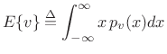 |
(C.12) |
where
Example:
Let the random variable ![]() be uniformly distributed between
be uniformly distributed between
![]() and
and ![]() , i.e.,
, i.e.,
![$\displaystyle p_v(x) = \left\{\begin{array}{ll} \frac{1}{b-a}, & a\leq x \leq b \\ [5pt] 0, & \hbox{otherwise}. \\ \end{array} \right.$](http://www.dsprelated.com/josimages_new/sasp2/img2645.png) |
(C.13) |
Then the expected value of
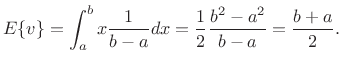 |
(C.14) |
Thus, the expected value of a random variable uniformly distributed between
For a stochastic process, which is simply a sequence of random
variables, ![]() means the expected value of
means the expected value of ![]() over
``all realizations'' of the random process
over
``all realizations'' of the random process ![]() . This is also
called an ensemble average. In other words, for each ``roll of
the dice,'' we obtain an entire signal
. This is also
called an ensemble average. In other words, for each ``roll of
the dice,'' we obtain an entire signal
![]() , and to compute
, and to compute ![]() , say, we average
together all of the values of
, say, we average
together all of the values of ![]() obtained for all ``dice rolls.''
obtained for all ``dice rolls.''
For a stationary random process
![]() , the random variables
, the random variables ![]() which make it up
are identically distributed. As a result, we may normally compute
expected values by averaging over time within a single
realization of the random process, instead of having to average
``vertically'' at a single time instant over many realizations of the
random process.C.2 Denote time averaging by
which make it up
are identically distributed. As a result, we may normally compute
expected values by averaging over time within a single
realization of the random process, instead of having to average
``vertically'' at a single time instant over many realizations of the
random process.C.2 Denote time averaging by
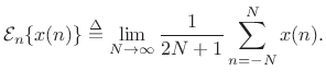 |
(C.15) |
Then, for a stationary random processes, we have
We are concerned only with stationary stochastic processes in this book. While the statistics of noise-like signals must be allowed to evolve over time in high quality spectral models, we may require essentially time-invariant statistics within a single frame of data in the time domain. In practice, we choose our spectrum analysis window short enough to impose this. For audio work, 20 ms is a typical choice for a frequency-independent frame length.C.3 In a multiresolution system, in which the frame length can vary across frequency bands, several periods of the band center-frequency is a reasonable choice. As discussed in §5.5.2, the minimum number of periods required under the window for resolution of spectral peaks depends on the window type used.
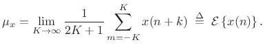
Mean
Definition:
The mean of a stochastic process ![]() at time
at time ![]() is defined as
the expected value of
is defined as
the expected value of ![]() :
:
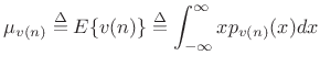 |
(C.16) |
where
For a stationary stochastic process ![]() , the mean is given by
the expected value of
, the mean is given by
the expected value of ![]() for any
for any ![]() . I.e.,
. I.e.,
![]() for all
for all ![]() .
.
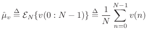
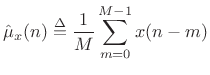
Sample Mean
Definition:
The sample mean of a set of ![]() samples from a particular
realization of a stationary stochastic process
samples from a particular
realization of a stationary stochastic process ![]() is defined
as the average of those samples:
is defined
as the average of those samples:
 |
(C.17) |
For a stationary stochastic process
| (C.18) |
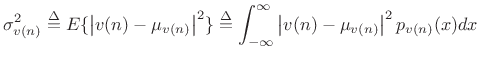
Variance
Definition:
The variance or second central moment of a stochastic
process ![]() at time
at time ![]() is defined as the expected value of
is defined as the expected value of
![]() :
:
 |
(C.19) |
where
For a stationary stochastic process ![]() , the variance is given
by the expected value of
, the variance is given
by the expected value of
![]() for any
for any ![]() .
.
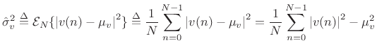
Sample Variance
Definition:
The sample variance of a set of ![]() samples from a particular
realization of a stationary stochastic process
samples from a particular
realization of a stationary stochastic process ![]() is defined
as average squared magnitude after removing the known mean:
is defined
as average squared magnitude after removing the known mean:
 |
(C.20) |
The sample variance is a unbiased estimator of the true variance when the mean is known, i.e.,
| (C.21) |
This is easy to show by taking the expected value:
When the mean is unknown, the sample mean is used in its place:
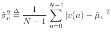 |
(C.23) |
The normalization by
Correlation Analysis
Correlation analysis applies only to stationary stochastic processes (§C.1.5).
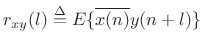
Cross-Correlation
Definition: The cross-correlation of two signals ![]() and
and
![]() may be defined by
may be defined by
 |
(C.24) |
I.e., it is the expected value (§C.1.6) of the lagged products in random signals
Cross-Power Spectral Density
The DTFT of the cross-correlation is called the cross-power spectral density, or ``cross-spectral density,'' ``cross-power spectrum,'' or even simply ``cross-spectrum.''
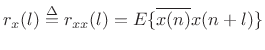
Autocorrelation
The cross-correlation of a signal with itself gives the autocorrelation function of that signal:
 |
(C.25) |
Note that the autocorrelation function is Hermitian:
When
Sample Autocorrelation
See §6.4.
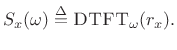
Power Spectral Density
The Fourier transform of the autocorrelation function ![]() is
called the power spectral density (PSD), or power
spectrum, and may be denoted
is
called the power spectral density (PSD), or power
spectrum, and may be denoted
When the signal
Sample Power Spectral Density
See §6.5.
White Noise
Definition:
To say that ![]() is a white noise means merely that
successive samples are uncorrelated:
is a white noise means merely that
successive samples are uncorrelated:
![$\displaystyle E\{v(n)v(n+m)\} = \left\{\begin{array}{ll} \sigma_v^2, & m=0 \\ [5pt] 0, & m\neq 0 \\ \end{array} \right. \isdef \sigma_v^2 \delta(m) \protect$](http://www.dsprelated.com/josimages_new/sasp2/img2676.png)
where
In other words, the autocorrelation function of white noise is an impulse at lag 0. Since the power spectral density is the Fourier transform of the autocorrelation function, the PSD of white noise is a constant. Therefore, all frequency components are equally present--hence the name ``white'' in analogy with white light (which consists of all colors in equal amounts).
Making White Noise with Dice
An example of a digital white noise generator is the sum of a pair of
dice minus 7. We must subtract 7 from the sum to make it zero
mean. (A nonzero mean can be regarded as a deterministic component at
dc, and is thus excluded from any pure noise signal for our purposes.)
For each roll of the dice, a number between
![]() and
and ![]() is generated. The numbers are distributed binomially between
is generated. The numbers are distributed binomially between ![]() and
and
![]() , but this has nothing to do with the whiteness of the number
sequence generated by successive rolls of the dice. The value of a
single die minus
, but this has nothing to do with the whiteness of the number
sequence generated by successive rolls of the dice. The value of a
single die minus ![]() would also generate a white noise sequence,
this time between
would also generate a white noise sequence,
this time between ![]() and
and ![]() and distributed with equal
probability over the six numbers
and distributed with equal
probability over the six numbers
![$\displaystyle \left[-\frac{5}{2}, -\frac{3}{2}, -\frac{1}{2}, \frac{1}{2}, \frac{3}{2}, \frac{5}{2}\right].$](http://www.dsprelated.com/josimages_new/sasp2/img2686.png) |
(C.27) |
To obtain a white noise sequence, all that matters is that the dice are sufficiently well shaken between rolls so that successive rolls produce independent random numbers.C.4
Independent Implies Uncorrelated
It can be shown that independent zero-mean random numbers are also uncorrelated, since, referring to (C.26),
![$\displaystyle E\{\overline{v(n)}v(n+m)\} = \left\{\begin{array}{ll} E\{\left\vert v(n)\right\vert^2\} = \sigma_v^2, & m=0 \\ [5pt] E\{\overline{v(n)}\}\cdot E\{v(n+m)\}=0, & m\neq 0 \\ \end{array} \right. \isdef \sigma_v^2 \delta(m)$](http://www.dsprelated.com/josimages_new/sasp2/img2689.png) |
(C.28) |
For Gaussian distributed random numbers, being uncorrelated also implies independence [201]. For related discussion illustrations, see §6.3.
Estimator Variance
As mentioned in §6.12, the pwelch function in Matlab
and Octave offer ``confidence intervals'' for an estimated power
spectral density (PSD). A confidence interval encloses the
true value with probability ![]() (the confidence level). For
example, if
(the confidence level). For
example, if ![]() , then the confidence level is
, then the confidence level is ![]() .
.
This section gives a first discussion of ``estimator variance,'' particularly the variance of sample means and sample variances for stationary stochastic processes.
Sample-Mean Variance
The simplest case to study first is the sample mean:
 |
(C.29) |
Here we have defined the sample mean at time
| (C.30) |
or
 |
(C.31) |
Now assume
Var![$\displaystyle \left\{x(n)\right\} \isdefs {\cal E}\left\{[x(n)-\mu_x]^2\right\} \eqsp {\cal E}\left\{x^2(n)\right\} \eqsp \sigma_x^2$](http://www.dsprelated.com/josimages_new/sasp2/img2697.png) |
(C.32) |
Then the variance of our sample-mean estimator
![]() can be calculated as follows:
can be calculated as follows:
![\begin{eqnarray*}
\mbox{Var}\left\{\hat{\mu}_x(n)\right\} &\isdef & {\cal E}\left\{\left[\hat{\mu}_x(n)-\mu_x \right]^2\right\}
\eqsp {\cal E}\left\{\hat{\mu}_x^2(n)\right\}\\
&=&{\cal E}\left\{\frac{1}{M}\sum_{m_1=0}^{M-1} x(n-m_1)\,
\frac{1}{M}\sum_{m_2=0}^{M-1} x(n-m_2)\right\}\\
&=&\frac{1}{M^2}\sum_{m_1=0}^{M-1}\sum_{m_2=0}^{M-1}
{\cal E}\left\{x(n-m_1) x(n-m_2)\right\}\\
&=&\frac{1}{M^2}\sum_{m_1=0}^{M-1}\sum_{m_2=0}^{M-1}
r_x(\vert m_1-m_2\vert)
\end{eqnarray*}](http://www.dsprelated.com/josimages_new/sasp2/img2699.png)
where we used the fact that the time-averaging operator
![]() is
linear, and
is
linear, and ![]() denotes the unbiased autocorrelation of
denotes the unbiased autocorrelation of ![]() .
If
.
If ![]() is white noise, then
is white noise, then
![]() , and we obtain
, and we obtain
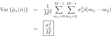
We have derived that the variance of the ![]() -sample running average of
a white-noise sequence
-sample running average of
a white-noise sequence ![]() is given by
is given by
![]() , where
, where
![]() denotes the variance of
denotes the variance of ![]() . We found that the
variance is inversely proportional to the number of samples used to
form the estimate. This is how averaging reduces variance in general:
When averaging
. We found that the
variance is inversely proportional to the number of samples used to
form the estimate. This is how averaging reduces variance in general:
When averaging ![]() independent (or merely uncorrelated) random
variables, the variance of the average is proportional to the variance
of each individual random variable divided by
independent (or merely uncorrelated) random
variables, the variance of the average is proportional to the variance
of each individual random variable divided by ![]() .
.
Sample-Variance Variance
Consider now the sample variance estimator
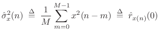 |
(C.33) |
where the mean is assumed to be
![$ {\cal E}\left\{[\hat{\sigma}_x^2(n)]^2\right\} = {\cal E}\left\{\hat{r}_{x(n)}^2(0)\right\} = \sigma_x^2$](http://www.dsprelated.com/josimages_new/sasp2/img2708.png) .
The variance of this estimator is then given by
.
The variance of this estimator is then given by
![\begin{eqnarray*}
\mbox{Var}\left\{\hat{\sigma}_x^2(n)\right\} &\isdef & {\cal E}\left\{[\hat{\sigma}_x^2(n)-\sigma_x^2]^2\right\}\\
&=& {\cal E}\left\{[\hat{\sigma}_x^2(n)]^2-\sigma_x^4\right\}
\end{eqnarray*}](http://www.dsprelated.com/josimages_new/sasp2/img2709.png)
where
![\begin{eqnarray*}
{\cal E}\left\{[\hat{\sigma}_x^2(n)]^2\right\} &=&
\frac{1}{M^2}\sum_{m_1=0}^{M-1}\sum_{m_1=0}^{M-1}{\cal E}\left\{x^2(n-m_1)x^2(n-m_2)\right\}\\
&=& \frac{1}{M^2}\sum_{m_1=0}^{M-1}\sum_{m_1=0}^{M-1}r_{x^2}(\vert m_1-m_2\vert)
\end{eqnarray*}](http://www.dsprelated.com/josimages_new/sasp2/img2710.png)
The autocorrelation of ![]() need not be simply related to that of
need not be simply related to that of
![]() . However, when
. However, when ![]() is assumed to be Gaussian white
noise, simple relations do exist. For example, when
is assumed to be Gaussian white
noise, simple relations do exist. For example, when
![]() ,
,
| (C.34) |
by the independence of
When ![]() is assumed to be Gaussian white noise, we have
is assumed to be Gaussian white noise, we have
![$\displaystyle {\cal E}\left\{x^2(n-m_1)x^2(n-m_2)\right\} = \left\{\begin{array}{ll} \sigma_x^4, & m_1\ne m_2 \\ [5pt] 3\sigma_x^4, & m_1=m_2 \\ \end{array} \right.$](http://www.dsprelated.com/josimages_new/sasp2/img2721.png) |
(C.35) |
so that the variance of our estimator for the variance of Gaussian white noise is
Var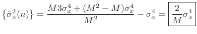 |
(C.36) |
Again we see that the variance of the estimator declines as
The same basic analysis as above can be used to estimate the variance of the sample autocorrelation estimates for each lag, and/or the variance of the power spectral density estimate at each frequency.
As mentioned above, to obtain a grounding in statistical signal processing, see references such as [201,121,95].
Next Section:
Gaussian Function Properties
Previous Section:
Selected Continuous Fourier Theorems


