


Computing 
Our goal is to find the allpass coefficient ![]() such that the
frequency mapping
such that the
frequency mapping
best approximates the Bark scale
Using squared frequency errors to gauge the fit between
![]() and
its Bark-warped counterpart, the optimal mapping-parameter
and
its Bark-warped counterpart, the optimal mapping-parameter ![]() may
be written as
may
be written as
![$\displaystyle \rho ^*= \hbox{Arg}\left[\min_{\rho }\left\{\left\Vert\,a(\omega )- b(\omega )\,\right\Vert\right\}\right],
$](http://www.dsprelated.com/josimages_new/sasp2/img2886.png)
where

is nonlinear in
has a norm which is more amenable to minimization. The first issue we address is how the minimizers of
![\includegraphics[width=3in]{eps/eaec}](http://www.dsprelated.com/josimages_new/sasp2/img2893.png)
Denote by ![]() and
and ![]() the complex representations of the
frequencies
the complex representations of the
frequencies
![]() and
and
![]() on the unit circle,
on the unit circle,
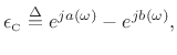
As seen in Fig.E.2, the absolute frequency error
The desired arc length error
Accordingly, essentially the same
The error
![]() is also nonlinear in the parameter
is also nonlinear in the parameter ![]() , and to find
its norm minimizer, an equation error is introduced, as is
common practice in developing solutions to nonlinear system
identification problems [152]. Consider mapping
the frequency
, and to find
its norm minimizer, an equation error is introduced, as is
common practice in developing solutions to nonlinear system
identification problems [152]. Consider mapping
the frequency
![]() via the allpass transformation
via the allpass transformation
![]() ,
,

Now, multiply (E.3.1) by the denominator
Rearranging terms, we have
where
It is shown in [269] that the optimal weighted least-squares conformal map parameter estimate is given by
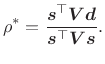
If the weighting matrix
![$\displaystyle \frac{\sum_{k=1}^K
v(\omega _k)
\sin\left[\frac{b(\omega_{k})-\omega_{k}}{2}\right]
\sin\left[\frac{b(\omega_{k})+\omega_{k}}{2}\right]
}{\sum_{k=1}^K
v(\omega _k)\sin^2\left[\frac{b(\omega_{k})+\omega_{k}}{2}\right]}$](http://www.dsprelated.com/josimages_new/sasp2/img2913.png) |
|||
![$\displaystyle \frac{\sum_{k=1}^{K}
v(\omega _k)
\left\{\cos\left[b(\omega_{k})\right]- \cos(\omega_{k})\right\}}{%
\sum_{k=1}^{K} v(\omega_{k}) \left\{\cos\left[b(\omega_{k}) + \omega_{k}\right]- 1\right\}}.$](http://www.dsprelated.com/josimages_new/sasp2/img2914.png) |
The kth diagonal element of an optimal diagonal weighting matrix
![]() is given by [269]
is given by [269]
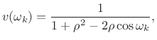
Note that the desired weighting depends on the unknown map parameter
![]() . To overcome this difficulty, we suggest first estimating
. To overcome this difficulty, we suggest first estimating
![]() using
using
![]() , where
, where
![]() denotes the identity matrix,
and then computing
denotes the identity matrix,
and then computing ![]() using the weighting (E.3.1) based on the
unweighted solution. This is analogous to the Steiglitz-McBride
algorithm for converting an equation-error minimizer to the more
desired ``output-error'' minimizer using an iteratively computed
weight function [151].
using the weighting (E.3.1) based on the
unweighted solution. This is analogous to the Steiglitz-McBride
algorithm for converting an equation-error minimizer to the more
desired ``output-error'' minimizer using an iteratively computed
weight function [151].
Next Section:
Optimal Frequency Warpings
Previous Section:
Gaussian Central Moments


