


Convolving with Long Signals
We saw that we can perform efficient convolution of two finite-length sequences using a Fast Fourier Transform (FFT). There are some situations, however, in which it is impractical to use a single FFT for each convolution operand:
- One or both of the signals being convolved is very long.
- The filter must operate in real time. (We can't wait until the input signal ends before providing an output signal.)
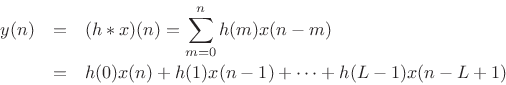
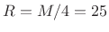
Thus, at every time ![]() , the output
, the output ![]() can be computed as a linear
combination of the current input sample
can be computed as a linear
combination of the current input sample ![]() and the current filter
state
and the current filter
state
![]() .
.
To obtain the benefit of high-speed FFT convolution when the input
signal is very long, we simply chop up the input signal ![]() into
blocks, and perform convolution on each block separately. The output
is then the sum of the separately filtered blocks. The blocks
overlap because of the ``ringing'' of the filter. For a
zero-phase filter, each block overlaps with both of its neighboring
blocks. For causal filters, each block overlaps only with its
neighbor to the right (the next block in time). The fact that signal
blocks overlap and must be added together (instead of simply abutted)
is the source of the name overlap-add method for FFT
convolution of long sequences [7,9].
into
blocks, and perform convolution on each block separately. The output
is then the sum of the separately filtered blocks. The blocks
overlap because of the ``ringing'' of the filter. For a
zero-phase filter, each block overlaps with both of its neighboring
blocks. For causal filters, each block overlaps only with its
neighbor to the right (the next block in time). The fact that signal
blocks overlap and must be added together (instead of simply abutted)
is the source of the name overlap-add method for FFT
convolution of long sequences [7,9].
The idea of processing input blocks separately can be extended also to
both operands of a convolution (both ![]() and
and ![]() in
in ![]() ). The
details are a straightforward extension of the single-block-signal
case discussed below.
). The
details are a straightforward extension of the single-block-signal
case discussed below.
When simple FFT convolution is being performed between a signal ![]() and FIR filter
and FIR filter ![]() , there is no reason to use a non-rectangular
window function on each input block. A rectangular window
length of
, there is no reason to use a non-rectangular
window function on each input block. A rectangular window
length of ![]() samples may advance
samples may advance ![]() samples for each successive
frame (hop size
samples for each successive
frame (hop size ![]() samples). In this case, the input blocks do not
overlap, while the output blocks overlap by the FIR filter length
(minus one sample). On the other hand, if nonlinear and/or time-varying
spectral modifications to be performed, then there are good reasons to
use a non-rectangular window function and a smaller hop size, as we
will develop below.
samples). In this case, the input blocks do not
overlap, while the output blocks overlap by the FIR filter length
(minus one sample). On the other hand, if nonlinear and/or time-varying
spectral modifications to be performed, then there are good reasons to
use a non-rectangular window function and a smaller hop size, as we
will develop below.
Overlap-Add Decomposition
Consider breaking an input signal ![]() into frames using a finite,
zero-phase, length
into frames using a finite,
zero-phase, length ![]() window
window ![]() . Then we may express the
. Then we may express the ![]() th
windowed data frame as
th
windowed data frame as
 |
(9.17) |
or
 |
(9.18) |
where

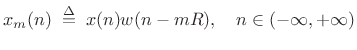
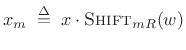
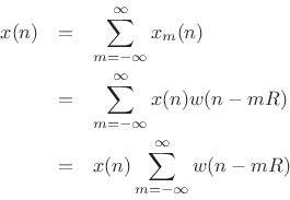
The hop size is the number of samples between the begin-times of adjacent frames. Specifically, it is the number of samples by which we advance each successive window.
Figure 8.8 shows an input signal (top) and three successive
windowed data frames using a length ![]() causal Hamming window and
50% overlap (
causal Hamming window and
50% overlap (![]() ).
).
![\includegraphics[width=\textwidth ]{eps/windsig}](http://www.dsprelated.com/josimages_new/sasp2/img1388.png)
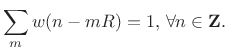
For frame-by-frame spectral processing to work, we must be able to
reconstruct ![]() from the individual overlapping frames, ideally by
simply summing them in their original time positions. This can be
written as
from the individual overlapping frames, ideally by
simply summing them in their original time positions. This can be
written as
Hence,
![]() if and only if
if and only if
 |
(9.19) |
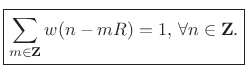
This is the constant-overlap-add (COLA)9.6 constraint for the FFT analysis window
![\includegraphics[width=3.5in]{eps/cola}](http://www.dsprelated.com/josimages_new/sasp2/img1392.png)
Figure 8.9 illustrates the appearance of 50% overlap-add for
the Bartlett (triangular) window. The Bartlett window is clearly COLA
for a wide variety of hop sizes, such as ![]() ,
, ![]() , and so on,
provided
, and so on,
provided ![]() is an integer (otherwise the underlying continuous
triangular window must be resampled). However, when using windows
defined in a library, the COLA condition should be carefully checked.
For example, the following Matlab/Octave script shows that there
is a problem with the standard Hamming window:
is an integer (otherwise the underlying continuous
triangular window must be resampled). However, when using windows
defined in a library, the COLA condition should be carefully checked.
For example, the following Matlab/Octave script shows that there
is a problem with the standard Hamming window:
M = 33;          % window length
R = (M-1)/2;     % hop size
N = 3*M;         % overlap-add span
w = hamming(M);  % window
z = zeros(N,1);  plot(z,'-k');  hold on;  s = z;
for so=0:R:N-M
  ndx = so+1:so+M;        % current window location
  s(ndx) = s(ndx) + w;    % window overlap-add
  wzp = z; wzp(ndx) = w;  % for plot only
  plot(wzp,'--ok');       % plot just this window
end
plot(s,'ok');  hold off;  % plot window overlap-add
The figure produced by this matlab code is shown in Fig.8.10. As can be seen, the equal end-points sum to form an impulse in each frame of the overlap-add.
![\includegraphics[width=3.5in]{eps/tolaq}](http://www.dsprelated.com/josimages_new/sasp2/img1395.png)
The Matlab window functions (such as hamming) have an optional second argument which can be either 'symmetric' (the default), or 'periodic'. The periodic case is equivalent to
w = hamming(M+1); % symmetric case
w = w(1:M);       % delete last sample for periodic case
The periodic variant solves the non-constant overlap-add problem for even
w = hamming(M); % symmetric case
w(1) = w(1)/2;  % repair constant-overlap-add for R=(M-1)/2
w(M) = w(M)/2;
Since different window types may add or subtract 1 to/from
- hamming(M)

.54 - .46*cos(2*pi*(0:M-1)'/(M-1));
gives constant overlap-add for ,
,  , etc.,
when endpoints are divided by 2 or one endpoint is zeroed
, etc.,
when endpoints are divided by 2 or one endpoint is zeroed
- hanning(M)
.5*(1 - cos(2*pi*(1:M)'/(M+1)));
does not give constant overlap-add for
,
but does for 
- blackman(M)
.42 - .5*cos(2*pi*m)' + .08*cos(4*pi*m)';
where m = (0:M-1)/(M-1), gives constant overlap-add for when
when  is odd and
  is an integer, and
  when
is even and
is integer.
when
is even and
is integer.
In summary, all windows obeying the constant-overlap-add constraint
will yield perfect reconstruction of the original signal ![]() from the
data frames
from the
data frames
![]() by overlap-add (OLA). There
is no constraint on window type, only that the window overlap-adds to
a constant for the hop size used. In particular,
by overlap-add (OLA). There
is no constraint on window type, only that the window overlap-adds to
a constant for the hop size used. In particular, ![]() always yields
a constant overlap-add for any window function. We will learn later
(§8.3.1) that there is also a simple frequency-domain test on
the window transform for the constant overlap-add property.
always yields
a constant overlap-add for any window function. We will learn later
(§8.3.1) that there is also a simple frequency-domain test on
the window transform for the constant overlap-add property.
To emphasize an earlier point, if simple time-invariant FIR filtering
is being implemented, and we don't need to work with the intermediate
STFT, it is most efficient to use the rectangular window with
hop size ![]() , and to set
, and to set ![]() , where
, where ![]() is the length of the
filter
is the length of the
filter ![]() and
and ![]() is a convenient FFT size. The optimum
is a convenient FFT size. The optimum ![]() for a
given
for a
given ![]() is an interesting exercise to work out.
is an interesting exercise to work out.
COLA Examples
So far we've seen the following constant-overlap-add examples:
- Rectangular window at 0% overlap (hop size
= window size
)
- Bartlett window at 50% overlap (
 )
(Since normally
is odd, ``
'' means ``R=(M-1)/2,''
etc.)
)
(Since normally
is odd, ``
'' means ``R=(M-1)/2,''
etc.)
- Hamming window at 50% overlap (
)
- Rectangular window at 50% overlap (
)
- Hamming window at 75% overlap (
 % hop size)
- Any member of the Generalized Hamming family at 50% overlap
- Any member of the Blackman family at 2/3 overlap (1/3 hop size);
e.g., blackman(33,'periodic'),

- Any member of the
 -term Blackman-Harris family with
 .
.
- Any window with R=1 (``sliding FFT'')
STFT of COLA Decomposition
To represent practical FFT implementations, it is preferable
to shift the ![]() frame back to the time origin:
frame back to the time origin:
 |
(9.20) |
This is summarized in Fig.8.11. Zero-based frames are needed because the leftmost input sample is assigned to time zero by FFT algorithms. In other words, a hopping FFT effectively redefines time zero on each hop. Thus, a practical STFT is a sequence of FFTs of the zero-based frames
![\begin{psfrags}
% latex2html id marker 21934\psfrag{x}{$x$}\psfrag{Zero-centered 3rd frame x_3: M = 64, R = M/2}%
{\normalsize Zero-centered 3rd frame $x_3$: $M = 64$, $R = M/2$}\psfrag{x_3}{$x_3$} % doesn't work\psfrag{xtilde_3}{${\tilde x}_3$}\begin{figure}[htbp]
\includegraphics[width=\twidth]{eps/shiftwin}
\caption{Input signal $x$\ (top), third frame
$x_3$\ in its natural time location (middle), and the third frame
shifted to time 0, ${\tilde x}_3$\ (bottom).}
\end{figure}
\end{psfrags}](http://www.dsprelated.com/josimages_new/sasp2/img1412.png)
Note that we may sample the DTFT of both ![]() and
and
![]() ,
because both are time-limited to
,
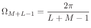
because both are time-limited to ![]() nonzero samples. The
minimum information-preserving sampling interval along the unit circle
in both cases is
nonzero samples. The
minimum information-preserving sampling interval along the unit circle
in both cases is
![]() . In practice, we often
oversample to some extent, using
. In practice, we often
oversample to some extent, using ![]() with
with ![]() instead. For
instead. For
![]() , we get
, we get
where
 . For
. For
Since
![]() , their transforms are related by the
shift theorem:
, their transforms are related by the
shift theorem:

where ![]() denotes modulo
denotes modulo ![]() indexing (appropriate since the
DTFTs have been sampled at intervals of
indexing (appropriate since the
DTFTs have been sampled at intervals of
![]() ).
).
Acyclic Convolution
Getting back to acyclic convolution, we may write it as
Since
![]() is time limited to
is time limited to
![]() (or
(or
![]() ),
),
![]() can be sampled at intervals of
can be sampled at intervals of
![]() without time aliasing. If
without time aliasing. If ![]() is time-limited to
is time-limited to
![]() , then
, then
![]() will be time limited to
will be time limited to ![]() . Therefore, we may sample
. Therefore, we may sample
![]() at intervals of
at intervals of
 |
(9.22) |
or less along the unit circle. This is the dual of the usual sampling theorem.
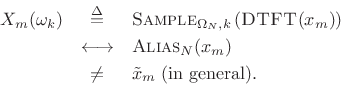
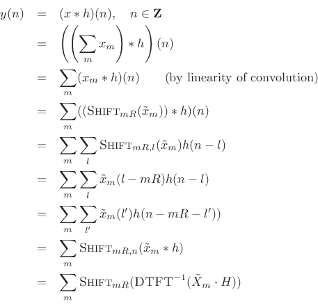
We conclude that practical FFT acyclic convolution may be carried out
using an FFT of any length ![]() satisfying
satisfying
| (9.23) |
where
![\begin{eqnarray*}
y(n) &=&
\sum_m \hbox{\sc Shift}_{mR,n} \left[\frac{1}{N} \sum_{k=0}^{N-1}
{\tilde H}(\omega_k) {\tilde X}_m(\omega_k) e^{j\omega_k n T}\right]\\
&=&
\sum_m \hbox{\sc Shift}_{mR,n}\left\{ \hbox{\sc IFFT}_N[\hbox{\sc FFT}_N({\tilde x}_m)\cdot \hbox{\sc FFT}_N(h)]\right\},
\end{eqnarray*}](http://www.dsprelated.com/josimages_new/sasp2/img1434.png)
where
![]() is the length
is the length ![]() DFT of the zero-padded
DFT of the zero-padded
![]() frame
frame
![]() , and
, and
![]() is the length
is the length ![]() DFT of
DFT of ![]() ,
also zero-padded out to length
,
also zero-padded out to length ![]() , with
, with
![]() .
.
Note that the terms in the outer sum overlap when ![]() even if
even if
![]() . In general, an LTI filtering by
. In general, an LTI filtering by ![]() increases
the amount of overlap among the frames.
increases
the amount of overlap among the frames.
This completes our derivation of FFT convolution between an
indefinitely long signal ![]() and a reasonably short FIR filter
and a reasonably short FIR filter
![]() (short enough that its zero-padded DFT can be practically
computed using one FFT).
(short enough that its zero-padded DFT can be practically
computed using one FFT).
The fast-convolution processor we have derived is a special case of the Overlap-Add (OLA) method for short-time Fourier analysis, modification, and resynthesis. See [7,9] for more details.
Example of Overlap-Add Convolution
Let's look now at a specific example of FFT convolution:
- Impulse-train test signal, 4000 Hz sampling-rate
- Length
 causal lowpass filter, 600 Hz cut-off
- Length
 rectangular window
- Hop size
 (no overlap)
We will work through the matlab for this example and display the results. First, the simulation parameters:
L = 31;         % FIR filter length in taps
fc = 600;       % lowpass cutoff frequency in Hz
fs = 4000;      % sampling rate in Hz

Nsig = 150;     % signal length in samples
period = round(L/3); % signal period in samples
FFT processing parameters:
M = L;                  % nominal window length
Nfft = 2^(ceil(log2(M+L-1))); % FFT Length
M = Nfft-L+1            % efficient window length
R = M;                  % hop size for rectangular window
Nframes = 1+floor((Nsig-M)/R);  % no. complete frames
Generate the impulse-train test signal:
sig = zeros(1,Nsig);
sig(1:period:Nsig) = ones(size(1:period:Nsig));
Design the lowpass filter using the window method:
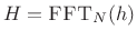
epsilon = .0001;     % avoids 0 / 0
nfilt = (-(L-1)/2:(L-1)/2) + epsilon;
hideal = sin(2*pi*fc*nfilt/fs) ./ (pi*nfilt);
w = hamming(L); % FIR filter design by window method
h = w' .* hideal; % window the ideal impulse response

hzp = [h zeros(1,Nfft-L)];  % zero-pad h to FFT size
H = fft(hzp);               % filter frequency response
Carry out the overlap-add FFT processing:
y = zeros(1,Nsig + Nfft); % allocate output+'ringing' vector
for m = 0:(Nframes-1)
    index = m*R+1:min(m*R+M,Nsig); % indices for the mth frame
    xm = sig(index);  % windowed mth frame (rectangular window)
    xmzp = [xm zeros(1,Nfft-length(xm))]; % zero pad the signal
    Xm = fft(xmzp);
    Ym = Xm .* H;               % freq domain multiplication
    ym = real(ifft(Ym))         % inverse transform
    outindex = m*R+1:(m*R+Nfft);
    y(outindex) = y(outindex) + ym; % overlap add
end
The time waveforms for the first three frames (![]() ) are shown in
Figures 8.12 through 8.14. Notice how the causal linear-phase filtering results
in an overall signal delay by half the filter length. Also, note how
frames 0 and 2 contain four impulses, while frame 1 only happens to
catch three; this causes no difficulty, and the filtered result remains
correct by superposition.
) are shown in
Figures 8.12 through 8.14. Notice how the causal linear-phase filtering results
in an overall signal delay by half the filter length. Also, note how
frames 0 and 2 contain four impulses, while frame 1 only happens to
catch three; this causes no difficulty, and the filtered result remains
correct by superposition.
![\includegraphics[width=0.8\twidth]{eps/ola0}](http://www.dsprelated.com/josimages_new/sasp2/img1443.png)
![\includegraphics[width=0.8\twidth]{eps/ola1}](http://www.dsprelated.com/josimages_new/sasp2/img1444.png)
![\includegraphics[width=0.8\twidth]{eps/ola2}](http://www.dsprelated.com/josimages_new/sasp2/img1445.png)
Summary of Overlap-Add FFT Processing
Overlap-add FFT processors provide efficient implementations for FIR filters longer than 100 or so taps on single CPUs. Specifically, we ended up with:
![$\displaystyle y = \sum_{m=-\infty}^\infty \hbox{\sc Shift}_{mR} \left( \hbox{\sc DFT}_N^{-1} \left\{ H \cdot \hbox{\sc DFT}_N\left[\hbox{\sc Shift}_{-mR}(x)\cdot w \right]\right\}\right)$](http://www.dsprelated.com/josimages_new/sasp2/img1446.png) |
(9.24) |
where
- (1)
- Extract the
 th length
frame of data at time
th length
frame of data at time  .
.
- (2)
- Shift it to the base time interval
![$ [0,M-1]$](http://www.dsprelated.com/josimages_new/sasp2/img1448.png) (or
(or
![$ [-(M-1)/2,(M-1)/2]$](http://www.dsprelated.com/josimages_new/sasp2/img1426.png) ).
).
- (3)
- Optionally apply a length
analysis window
 (causal or zero phase, as preferred). For simple LTI filtering,
the rectangular window is fine.
(causal or zero phase, as preferred). For simple LTI filtering,
the rectangular window is fine.
- (4)
- Zero-pad the windowed data out to the FFT size
 (a power of 2),
such that
(a power of 2),
such that
 , where
is the FIR filter length.
, where
is the FIR filter length.
- (5)
- Take the
-point FFT.
- (6)
- Apply the filter frequency-response
 as a
windowing operation in the frequency domain.
as a
windowing operation in the frequency domain.
- (7)
- Take the
-point inverse FFT.
- (8)
- Shift the origin of the
-point result out to sample
where it belongs.
- (9)
- Sum into the output buffer containing the results from prior frames (OLA step).
A second condition is that the analysis window be COLA at the hop size used:
 |
(9.25) |
Next Section:
Dual of Constant Overlap-Add
Previous Section:
Convolution of Short Signals


