


Effect of Windowing
Let's look at a simple example of windowing to demonstrate what happens when we turn an infinite-duration signal into a finite-duration signal through windowing.
We begin with a sampled complex sinusoid:
| (6.14) |
A portion of the real part,
![\includegraphics[width=0.6\twidth]{eps/infDurSin}](http://www.dsprelated.com/josimages_new/sasp2/img931.png)
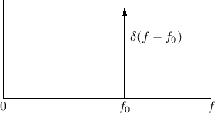
The Fourier transform of this infinite-duration signal is a delta
function at
![]() . I.e.,
. I.e.,
![]() , as indicated in Fig.5.4.
, as indicated in Fig.5.4.
The windowed signal is
| (6.15) |
as shown in Fig.5.5. (Note carefully the difference between
![\includegraphics[width=4in,height=2in]{eps/windowedSin}](http://www.dsprelated.com/josimages_new/sasp2/img934.png)
The convolution theorem (§2.3.5) tells
us that our multiplication in the time domain results in a convolution
in the frequency domain. Hence, we will obtain the convolution of
![]() with the Fourier transform of the window
with the Fourier transform of the window
![]() . This is easy since the delta function is the identity
element under convolution (
. This is easy since the delta function is the identity
element under convolution (
![]() ). However, since our
delta function is at frequency
). However, since our
delta function is at frequency
![]() , the
convolution shifts the window transform out to that frequency:
, the
convolution shifts the window transform out to that frequency:
| (6.16) |
This is shown in Fig.5.6.
![\includegraphics[width=\twidth]{eps/windowedSinSpec}](http://www.dsprelated.com/josimages_new/sasp2/img938.png) |
From comparing Fig.5.6 with the ideal sinusoidal
spectrum in Fig.5.4 (an impulse at frequency ![]() ),
we can make some observations:
),
we can make some observations:
- Windowing in the time domain resulted in a ``smearing''
or ``smoothing'' in the frequency domain. In particular, the
infinitely thin delta function has been replaced by the ``main lobe''
of the window transform. We need to be aware of this if we are trying
to resolve sinusoids which are close together in frequency.
- Windowing also introduced side lobes. This is important
when we are trying to resolve low amplitude sinusoids in the presence
of higher amplitude signals.
- A sinusoid at amplitude
 , frequency
  , and phase
 manifests (in practical spectrum analysis) as a
window transform shifted out to frequency
, and scaled
by
manifests (in practical spectrum analysis) as a
window transform shifted out to frequency
, and scaled
by
 .
.
As a result of the last point above, the ideal window transform is an impulse in the frequency domain. Since this cannot be achieved in practice, we try to find spectrum-analysis windows which approximate this ideal in some optimal sense. In particular, we want side-lobes that are as close to zero as possible, and we want the main lobe to be as tall and narrow as possible. (Since absolute scalings are normally arbitrary in signal processing, ``tall'' can be defined as the ratio of main-lobe amplitude to side-lobe amplitude--or main-lobe energy to side-lobe energy, etc.) There are many alternative formulations for ``approximating an impulse'', and each such formulation leads to a particular spectrum-analysis window which is optimal in that sense. In addition to these windows, there are many more which arise in other applications. Many commonly used window types are summarized in Chapter 3.
Frequency Resolution
The frequency resolution of a spectrum-analysis window is determined by its main-lobe width (Chapter 3) in the frequency domain, where a typical main lobe is illustrated in Fig.5.6 (top). For maximum frequency resolution, we desire the narrowest possible main-lobe width, which calls for the rectangular window (§3.1), the transform of which is shown in Fig.3.3. When we cannot be fooled by the large side-lobes of the rectangular window transform (e.g., when the sinusoids under analysis are known to be well separated in frequency), the rectangular window truly is the optimal window for the estimation of frequency, amplitude, and phase of a sinusoid in the presence of stationary noise [230,120,121].
The rectangular window has only one parameter (aside from amplitude)--its length. The next section looks at the effect of an increased window length on our ability to resolve two sinusoids.
Two Cosines (``In-Phase'' Case)
Figure 5.7 shows a spectrum analysis of two cosines
| (6.17) |
where
 ).
The length
).
The length
![\includegraphics[width=\twidth]{eps/resolvedSines}](http://www.dsprelated.com/josimages_new/sasp2/img951.png)
The longest window (![]() ) resolves the sinusoids very well, while
the shortest case (
) resolves the sinusoids very well, while
the shortest case (![]() ) does not resolve them at all (only one
``lump'' appears in the spectrum analysis). In difference-frequency
cycles, the analysis windows are two cycles and half a cycle in these
cases, respectively. It can be debated whether or not the other two
cases are resolved, and we will return to them shortly.
) does not resolve them at all (only one
``lump'' appears in the spectrum analysis). In difference-frequency
cycles, the analysis windows are two cycles and half a cycle in these
cases, respectively. It can be debated whether or not the other two
cases are resolved, and we will return to them shortly.
One Sine and One Cosine ``Phase Quadrature'' Case
Figure 5.8 shows a similar spectrum analysis of two sinusoids
| (6.18) |
using the same frequency separation and window lengths. However, now the sinusoids are 90 degrees out of phase (one sine and one cosine). Curiously, the top-left case (
![\includegraphics[width=\twidth]{eps/resolvedSinesB}](http://www.dsprelated.com/josimages_new/sasp2/img956.png)
Figure 5.9 shows the same plots as in Fig.5.8, but overlaid. From this we can see that the peak locations are biased in under-resolved cases, both in amplitude and frequency.
![\includegraphics[width=\textwidth ]{eps/resolvedSinesC2C}](http://www.dsprelated.com/josimages_new/sasp2/img957.png)
The preceding figures suggest that, for a rectangular window of length
![]() , two sinusoids are well resolved when they are separated in
frequency by
, two sinusoids are well resolved when they are separated in
frequency by
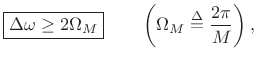 |
(6.19) |
where the frequency-separation
 |
(6.20) |
where the
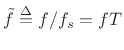 denotes normalized frequency in
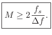
cycles per sample. In Hz, we have
denotes normalized frequency in
cycles per sample. In Hz, we have
 |
(6.21) |
or
 |
(6.22) |
Note that
A more detailed study [1] reveals that ![]() cycles
of the difference-frequency is sufficient to enable fully accurate
peak-frequency measurement under the rectangular window by means of
finding FFT peaks. In §5.5.2 below, additional minimum duration
specifications for resolving closely spaced sinusoids are given for
other window types as well.
cycles
of the difference-frequency is sufficient to enable fully accurate
peak-frequency measurement under the rectangular window by means of
finding FFT peaks. In §5.5.2 below, additional minimum duration
specifications for resolving closely spaced sinusoids are given for
other window types as well.
In principle, we can resolve arbitrarily small frequency separations, provided
- there is no noise, and
- we are sure we are looking at the sum of two ideal sinusoids under the window.
The rectangular window provides an abrupt transition at its edge. While it remains the optimal window for sinusoidal peak estimation, it is by no means optimal in all spectrum analysis and/or signal processing applications involving spectral processing. As discussed in Chapter 3, windows with a more gradual transition to zero have lower side-lobe levels, and this is beneficial for spectral displays and various signal processing applications based on FFT methods. We will encounter such applications in later chapters.
Next Section:
Resolving Sinusoids
Previous Section:
Spectrum of a Windowed Sinusoid


