


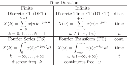
Fourier Transforms for Continuous/Discrete Time/Frequency
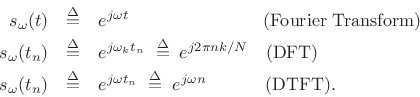
The Fourier transform can be defined for signals which are
- discrete or continuous in time, and
- finite or infinite in duration.
- discrete or continuous in frequency, and
- finite or infinite in bandwidth.
Reference [264] develops the DFT in detail--the discrete-time, discrete-frequency case. In the DFT, both the time and frequency axes are finite in length.
Table 2.1 (next page) summarizes the four Fourier-transform cases corresponding to discrete or continuous time and/or frequency.
 |
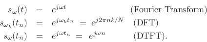
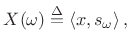
In all four cases, the Fourier transform can be interpreted as
the inner product of the signal ![]() with a complex sinusoid at
radian frequency
with a complex sinusoid at
radian frequency ![]() [264]:
[264]:
| (3.1) |
where
In spectral modeling of audio, we usually deal with indefinitely long signals. Fourier analysis of an indefinitely long discrete-time signal is carried out using the Discrete Time Fourier Transform (DTFT).3.1Below, the DTFT is defined, and selected Fourier theorems are stated and proved for the DTFT case. Additionally, for completeness, the Fourier Transform (FT) is defined, and selected FT theorems are stated and proved as well. Theorems for the DFT case are detailed in [264].3.2
Discrete Time Fourier Transform (DTFT)
The Discrete Time Fourier Transform (DTFT) can be viewed as the
limiting form of the DFT when its length ![]() is allowed to approach
infinity:
is allowed to approach
infinity:
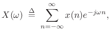 |
(3.2) |
where
The inverse DTFT is
 |
(3.3) |
which can be derived in a manner analogous to the derivation of the inverse DFT [264].
Instead of operating on sampled signals of length ![]() (like the DFT),
the DTFT operates on sampled signals
(like the DFT),
the DTFT operates on sampled signals ![]() defined over all integers
defined over all integers
![]() .
.
Unlike the DFT, the DTFT frequencies form a continuum. That
is, the DTFT is a function of continuous frequency
![]() , while the DFT is a function of discrete
frequency
, while the DFT is a function of discrete
frequency ![]() ,
,
![]() . The DFT frequencies
. The DFT frequencies
![]() ,
,
![]() , are given by the angles of
, are given by the angles of ![]() points
uniformly distributed along the unit circle in the complex
plane. Thus, as
points
uniformly distributed along the unit circle in the complex
plane. Thus, as
![]() , a continuous
frequency axis must result in the limit along the unit circle. The
axis is still finite in length, however, because the time domain
remains sampled.
, a continuous
frequency axis must result in the limit along the unit circle. The
axis is still finite in length, however, because the time domain
remains sampled.
Fourier Transform (FT) and Inverse
The Fourier transform of a signal
![]() ,
,
![]() , is defined as
, is defined as
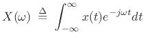
and its inverse is given by
Thus, the Fourier transform is defined for continuous time and continuous frequency, both unbounded. As a result, mathematical questions such as existence and invertibility are most difficult for this case. In fact, such questions fueled decades of confusion in the history of harmonic analysis (see Appendix G).
Existence of the Fourier Transform
Conditions for the existence of the Fourier transform are
complicated to state in general [36], but it is sufficient
for ![]() to be absolutely integrable, i.e.,
to be absolutely integrable, i.e.,
 |
(3.6) |
This requirement can be stated as
 |
(3.7) |
or,
There is never a question of existence, of course, for Fourier transforms of real-world signals encountered in practice. However, idealized signals, such as sinusoids that go on forever in time, do pose normalization difficulties. In practical engineering analysis, these difficulties are resolved using Dirac's ``generalized functions'' such as the impulse (also loosely called the delta function), discussed in §B.10.
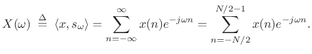
Fourier Theorems for the DTFT
This section states and proves selected Fourier theorems for the DTFT. A more complete list for the DFT case is given in [264].3.4Since this material was originally part of an appendix, it is relatively dry reading. Feel free to skip to the next chapter and refer back as desired when a theorem is invoked.
As introduced in §2.1 above, the Discrete-Time Fourier Transform (DTFT) may be defined as
 |
(3.8) |
We say that
Linearity of the DTFT
| (3.9) |
or
| (3.10) |
where
Proof:
We have
![\begin{eqnarray*}
\hbox{\sc DTFT}_\omega(\alpha x_1 + \beta x_2)
& \isdef & \sum_{n=-\infty}^{\infty}[\alpha x_1(n) + \beta x_2(n)]e^{-j\omega n}\\
&=& \alpha\sum_{n=-\infty}^{\infty}x_1(n)e^{-j\omega n} + \beta \sum_{n=-\infty}^{\infty}x_2(n)e^{-j\omega n}\\
&\isdef & \alpha X_1(\omega) + \beta X_2(\omega)
\end{eqnarray*}](http://www.dsprelated.com/josimages_new/sasp2/img126.png)
One way to describe the linearity property is to observe that the Fourier transform ``commutes with mixing.''
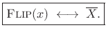
Time Reversal
For any complex signal ![]() ,
,
![]() , we have
, we have
| (3.11) |
where
 .
.
Proof:
![\begin{eqnarray*}
\hbox{\sc DTFT}_\omega(\hbox{\sc Flip}(x))
&\isdef & \sum_{n=-\infty}^{\infty} x(-n)e^{-j\omega n}
\eqsp \sum_{m=\infty}^{-\infty} x(m)e^{-j(-\omega) m}
\eqsp X(-\omega) \\ [5pt]
&\isdef & \hbox{\sc Flip}_\omega(X)
\end{eqnarray*}](http://www.dsprelated.com/josimages_new/sasp2/img130.png)
Arguably,
![]() should include complex conjugation. Let
should include complex conjugation. Let
 |
(3.12) |
denote such a definition. Then in this case we have
 |
(3.13) |
Proof:
 |
(3.14) |
In the typical special case of real signals (
![]() ), we have
), we have
![]() so that
so that
 |
(3.15) |
That is, time-reversing a real signal conjugates its spectrum.
Symmetry of the DTFT for Real Signals
Most (if not all) of the signals we deal with in practice are real signals. Here we note some spectral symmetries associated with real signals.
DTFT of Real Signals
The previous section established that the spectrum ![]() of every real
signal
of every real
signal ![]() satisfies
satisfies
| (3.16) |
I.e.,
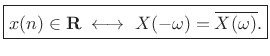 |
(3.17) |
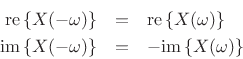
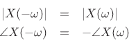
In other terms, if a signal
- The real part is even, while the imaginary part is odd:
- The magnitude is even, while the phase is odd:
Real Even (or Odd) Signals
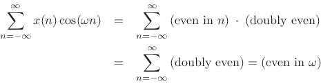
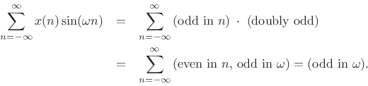
If a signal is even in addition to being real, then its DTFT is also real and even. This follows immediately from the Hermitian symmetry of real signals, and the fact that the DTFT of any even signal is real:
![\begin{eqnarray*}
\hbox{\sc DTFT}_\omega(x)
& \isdef & \sum_{n=-\infty}^{\infty}x(n) e^{-j\omega n}\\
& = & \sum_{n=-\infty}^{\infty}x(n) \left[\cos(\omega n) + j\sin(\omega n)\right]\\
& = & \sum_{n=-\infty}^{\infty}x(n) \cos(\omega n) + j\sum_{n=-\infty}^{\infty}x(n)\sin(\omega n)\\
& = & \sum_{n=-\infty}^{\infty}x(n) \cos(\omega n)\\
& = & \hbox{real and even}
\end{eqnarray*}](http://www.dsprelated.com/josimages_new/sasp2/img142.png)
This is true since cosine is even, sine is odd, even times even is even, even times odd is odd, and the sum over all samples of an odd signal is zero. I.e.,
and
If ![]() is real and even, the following are true:
is real and even, the following are true:
![\begin{eqnarray*}
\hbox{\sc Flip}(x) & = & x \qquad \hbox{($x(-n)=x(n)$)}\\
\overline{x} & = & x\\ [5pt]
\hbox{\sc Flip}(X) & = & X\\
\overline{X} & = & X\\
\angle X(\omega) & =& 0 \hbox{ or } \pi
\end{eqnarray*}](http://www.dsprelated.com/josimages_new/sasp2/img145.png)
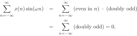
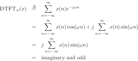
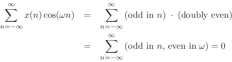
Similarly, if a signal is odd and real, then its DTFT is odd and purely imaginary. This follows from Hermitian symmetry for real signals, and the fact that the DTFT of any odd signal is imaginary.
where we used the fact that
and
Shift Theorem for the DTFT
We define the shift operator for sampled signals ![]() by
by
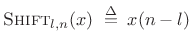 |
(3.18) |
where
The shift theorem states3.5
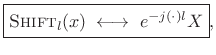 |
(3.19) |
or, in operator notation,
| (3.20) |
Proof:
![\begin{eqnarray*}
\hbox{\sc DTFT}_\omega[\hbox{\sc Shift}_l(x)] &\isdef & \sum_{n=-\infty}^{\infty}x(n-l) e^{-j \omega n} \\
&=& \sum_{m=-\infty}^{\infty} x(m) e^{-j \omega (m+l)}
\qquad(m\isdef n-l) \\
&=& \sum_{m=-\infty}^{\infty}x(m) e^{-j \omega m} e^{-j \omega l} \\
&=& e^{-j \omega l} \sum_{m=-\infty}^{\infty}x(m) e^{-j \omega m} \\
&\isdef & e^{-j \omega l} X(\omega)
\end{eqnarray*}](http://www.dsprelated.com/josimages_new/sasp2/img158.png)
Note that
![]() is a linear phase term, so called
because it is a linear function of frequency with slope equal to
is a linear phase term, so called
because it is a linear function of frequency with slope equal to ![]() :
:
| (3.21) |
The shift theorem gives us that multiplying a spectrum
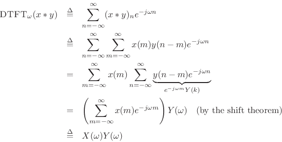
Convolution Theorem for the DTFT
The convolution of discrete-time signals ![]() and
and ![]() is defined
as
is defined
as
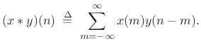 |
(3.22) |
This is sometimes called acyclic convolution to distinguish it from the cyclic convolution used for length
The convolution theorem is then
| (3.23) |
That is, convolution in the time domain corresponds to pointwise multiplication in the frequency domain.
Proof: The result follows immediately from interchanging the order
of summations associated with the convolution and DTFT:
Correlation Theorem for the DTFT
We define the correlation of discrete-time signals ![]() and
and ![]() by
by
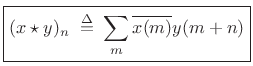
The correlation theorem for DTFTs is then

Proof:
where the last step follows from the convolution theorem of
§2.3.5 and the symmetry result
![]() of §2.3.2.
of §2.3.2.
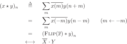
Autocorrelation
The autocorrelation of a signal ![]() is simply the
cross-correlation of
is simply the
cross-correlation of ![]() with itself:
with itself:
 |
(3.24) |
From the correlation theorem, we have
Note that this definition of autocorrelation is appropriate for signals having finite support (nonzero over a finite number of samples). For infinite-energy (but finite-power) signals, such as stationary noise processes, we define the sample autocorrelation to include a normalization suitable for this case (see Chapter 6 and Appendix C).
From the autocorrelation theorem we have that a digital-filter
impulse-response ![]() is that of a lossless allpass filter
[263] if and only if
is that of a lossless allpass filter
[263] if and only if
![]() .
In other words, the autocorrelation of the impulse-response of every
allpass filter is impulsive.
.
In other words, the autocorrelation of the impulse-response of every
allpass filter is impulsive.
Power Theorem for the DTFT
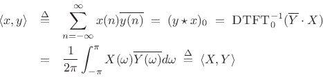
The inner product of two signals may be defined in the time domain by [264]
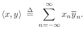 |
(3.25) |
The inner product of two spectra may be defined as
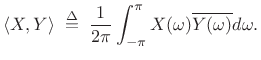 |
(3.26) |
Note that the frequency-domain inner product includes a normalization factor while the time-domain definition does not.
Using inner-product notation, the power theorem (or Parseval's theorem [202]) for DTFTs can be stated as follows:
| (3.27) |
That is, the inner product of two signals in the time domain equals the inner product of their respective spectra (a complex scalar in general).
When we consider the inner product of a signal with itself, we have the special case known as the energy theorem (or Rayleigh's energy theorem):
| (3.28) |
where
Proof:
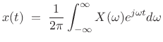
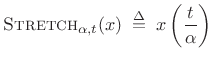
Stretch Operator
We define the stretch operator in the time domain by
![$\displaystyle \hbox{\sc Stretch}_{L,n}(x) \isdefs \left\{\begin{array}{ll} x\left(\frac{n}{L}\right), & n = 0\;(\hbox{\sc mod}\ L) \\ [5pt] 0, & \hbox{otherwise} \\ \end{array} \right..$](http://www.dsprelated.com/josimages_new/sasp2/img183.png) |
(3.29) |
In other terms, we stretch a sampled signal by the factor
![\includegraphics[width=4in]{eps/stretch2}](http://www.dsprelated.com/josimages_new/sasp2/img186.png)
In the literature on multirate filter banks (see Chapter 11), the
stretch operator is typically called instead the upsampling
operator. That is, stretching a signal by the factor of ![]() is called
upsampling the signal by the factor
is called
upsampling the signal by the factor ![]() . (See §11.1.1 for
the graphical symbol (
. (See §11.1.1 for
the graphical symbol (
![]() ) and associated discussion.) The
term ``stretch'' is preferred in this book because ``upsampling''
is easily confused with ``increasing the sampling rate''; resampling a
signal to a higher sampling rate is conceptually implemented by a
stretch operation followed by an ideal lowpass filter which moves the
inserted zeros to their properly interpolated values.
) and associated discussion.) The
term ``stretch'' is preferred in this book because ``upsampling''
is easily confused with ``increasing the sampling rate''; resampling a
signal to a higher sampling rate is conceptually implemented by a
stretch operation followed by an ideal lowpass filter which moves the
inserted zeros to their properly interpolated values.
Note that we could also call the stretch operator the scaling operator, to unify the terminology in the discrete-time case with that of the continuous-time case (§2.4.1 below).
Repeat (Scaling) Operator
We define the repeat operator in the frequency domain as
a scaling of frequency axis by some integer factor ![]() :
:
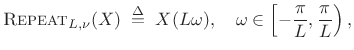 |
(3.30) |
where
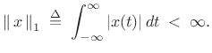
The repeat operator maps the entire unit circle (taken as ![]() to
to
![]() ) to a segment of itself
) to a segment of itself
![]() , centered about
, centered about
![]() , and repeated
, and repeated ![]() times. This is illustrated in Fig.2.2
for
times. This is illustrated in Fig.2.2
for ![]() .
.
![\begin{psfrags}
% latex2html id marker 7156\psfrag{w}{\Large $\omega$}\begin{figure}[htbp]
\includegraphics[width=\twidth]{eps/repeat2}
\caption{Illustration of the repeat operator.}
\end{figure}
\end{psfrags}](http://www.dsprelated.com/josimages_new/sasp2/img196.png)
Since the frequency axis is continuous and ![]() -periodic for DTFTs,
the repeat operator is precisely equivalent to a scaling operator for
the Fourier transform case (§B.4). We call it ``repeat''
rather than ``scale'' because we are restricting the scale factor to
positive integers, and because the name ``repeat'' describes more
vividly what happens to a periodic spectrum that is compressively
frequency-scaled over the unit circle by an integer factor.
-periodic for DTFTs,
the repeat operator is precisely equivalent to a scaling operator for
the Fourier transform case (§B.4). We call it ``repeat''
rather than ``scale'' because we are restricting the scale factor to
positive integers, and because the name ``repeat'' describes more
vividly what happens to a periodic spectrum that is compressively
frequency-scaled over the unit circle by an integer factor.
Stretch/Repeat (Scaling) Theorem
Using these definitions, we can compactly state the stretch theorem:
| (3.31) |
Proof:
![\begin{eqnarray*}
\hbox{\sc DTFT}_\omega[\hbox{\sc Stretch}_L(x)]
&\isdef & \sum_{n=-\infty}^{\infty}\hbox{\sc Stretch}_{L,n}(x)e^{-j\omega n}\\
&=& \sum_{m=-\infty}^{\infty}x(m)e^{-j\omega m L}\qquad \hbox{($m\isdef n/L$)}\\
&\isdef & X(\omega L)
\end{eqnarray*}](http://www.dsprelated.com/josimages_new/sasp2/img199.png)
As ![]() traverses the interval
traverses the interval
![]() ,
,
![]() traverses the unit circle
traverses the unit circle ![]() times, thus implementing the repeat
operation on the unit circle. Note also that when
times, thus implementing the repeat
operation on the unit circle. Note also that when ![]() , we have
, we have
![]() , so that dc always maps to dc. At half the sampling
rate
, so that dc always maps to dc. At half the sampling
rate
![]() , on the other hand, after the mapping, we may have
either
, on the other hand, after the mapping, we may have
either
![]() (
(![]() odd), or
odd), or ![]() (
(![]() even), where
even), where
![]() .
.
The stretch theorem makes it clear how to do
ideal sampling-rate conversion for integer upsampling ratios ![]() :
We first stretch the signal by the factor
:
We first stretch the signal by the factor ![]() (introducing
(introducing ![]() zeros
between each pair of samples), followed by an ideal lowpass
filter cutting off at
zeros
between each pair of samples), followed by an ideal lowpass
filter cutting off at ![]() . That is, the filter has a gain of 1
for
. That is, the filter has a gain of 1
for
![]() , and a gain of 0 for
, and a gain of 0 for
![]() . Such a system (if it were realizable) implements ideal bandlimited interpolation of the original signal by the factor
. Such a system (if it were realizable) implements ideal bandlimited interpolation of the original signal by the factor ![]() .
.
The stretch theorem is analogous to the scaling theorem for continuous Fourier transforms (introduced in §2.4.1 below).
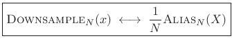
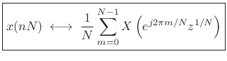
Downsampling and Aliasing
The downsampling operator
![]() selects every
selects every ![]() sample of a signal:
sample of a signal:
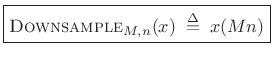 |
(3.32) |
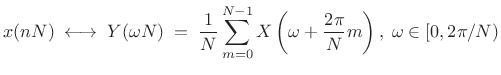
The aliasing theorem states that downsampling in time corresponds to aliasing in the frequency domain:
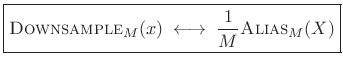 |
(3.33) |
where the
 |
(3.34) |
for
In z transform notation, the
![]() operator can be expressed as
[287]
operator can be expressed as
[287]
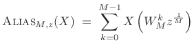 |
(3.35) |
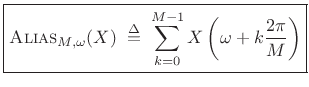
where
![$\displaystyle \hbox{\sc Alias}_{M,\omega}(X) \eqsp \sum_{k=0}^{M-1} X\left[e^{j\left(\frac{\omega}{M} + k\frac{2\pi}{M}\right)}\right], \quad -\pi\leq \omega < \pi.$](http://www.dsprelated.com/josimages_new/sasp2/img219.png) |
(3.36) |
The frequency scaling corresponds to having a sampling interval of
The aliasing theorem makes it clear that, in order to downsample by
factor ![]() without aliasing, we must first lowpass-filter the spectrum
to
without aliasing, we must first lowpass-filter the spectrum
to
![]() . This filtering (when ideal) zeroes out the
spectral regions which alias upon downsampling.
. This filtering (when ideal) zeroes out the
spectral regions which alias upon downsampling.
Note that any rational sampling-rate conversion factor
![]() may be implemented as an upsampling by the factor
may be implemented as an upsampling by the factor ![]() followed by
downsampling by the factor
followed by
downsampling by the factor ![]() [50,287].
Conceptually, a stretch-by-
[50,287].
Conceptually, a stretch-by-![]() is followed by a lowpass filter cutting
off at
is followed by a lowpass filter cutting
off at
![]() , followed by
downsample-by-
, followed by
downsample-by-![]() , i.e.,
, i.e.,
| (3.37) |
In practice, there are more efficient algorithms for sampling-rate conversion [270,135,78] based on a more direct approach to bandlimited interpolation.
Proof of Aliasing Theorem
To show:
or
From the DFT case [264], we know this is true when ![]() and
and ![]() are each complex sequences of length
are each complex sequences of length ![]() , in which case
, in which case ![]() and
and ![]() are length
are length ![]() . Thus,
. Thus,
 |
(3.38) |
where we have chosen to keep frequency samples
 |
(3.39) |
Replacing
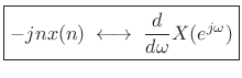
Differentiation Theorem Dual
Theorem: Let ![]() denote a signal with DTFT
denote a signal with DTFT
![]() , and let
, and let
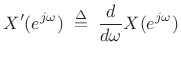 |
(3.40) |
denote the derivative of
where
Proof:
Using integration by parts, we obtain
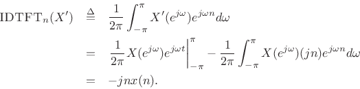
An alternate method of proof is given in §B.3.
Corollary: Perhaps a cleaner statement is as follows:

This completes our coverage of selected DTFT theorems. The next section adds some especially useful FT theorems having no precise counterpart in the DTFT (discrete-time) case.
Continuous-Time Fourier Theorems
Selected Fourier theorems for the continuous-time case are stated and proved in Appendix B. However, two are sufficiently important that we state them here.
Scaling Theorem
The scaling theorem (or similarity theorem) says that if
you horizontally ``stretch'' a signal by the factor ![]() in the
time domain, you ``squeeze'' and amplify its Fourier transform by the
same factor in the frequency domain. This is an important general
Fourier duality relationship:
in the
time domain, you ``squeeze'' and amplify its Fourier transform by the
same factor in the frequency domain. This is an important general
Fourier duality relationship:
Theorem: For all continuous-time functions ![]() possessing a Fourier
transform,
possessing a Fourier
transform,
where
and
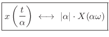 |
(3.41) |
Proof: See §B.4.
The scaling theorem is fundamentally restricted to the
continuous-time, continuous-frequency (Fourier transform) case. The
closest we come to the scaling theorem among the DTFT theorems
(§2.3) is the stretch (repeat) theorem
(page ![]() ). For this and other continuous-time Fourier
theorems, see Appendix B.
). For this and other continuous-time Fourier
theorems, see Appendix B.
Spectral Roll-Off
Definition: A function ![]() is said to be of order
is said to be of order
![]() if
there exist
if
there exist ![]() and some positive constant
and some positive constant ![]() such
that
such
that
![]() for all
for all
![]() .
.
Theorem: (Riemann Lemma):
If the derivatives up to order ![]() of a function
of a function ![]() exist and are
of bounded variation, then its Fourier Transform
exist and are
of bounded variation, then its Fourier Transform ![]() is
asymptotically of order
is
asymptotically of order
![]() , i.e.,
, i.e.,
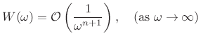 |
(3.42) |
Proof: See §B.18.
Spectral Interpolation
The need for spectral interpolation comes up in many situations. For example, we always use the DFT in practice, while conceptually we often prefer the DTFT. For time-limited signals, that is, signals which are zero outside some finite range, the DTFT can be computed from the DFT via spectral interpolation. Conversely, the DTFT of a time-limited signal can be sampled to obtain its DFT.3.7Another application of DFT interpolation is spectral peak estimation, which we take up in Chapter 5; in this situation, we start with a sampled spectral peak from a DFT, and we use interpolation to estimate the frequency of the peak more accurately than what we get by rounding to the nearest DFT bin frequency.
The following sections describe the theoretical and practical details of ideal spectral interpolation.
Ideal Spectral Interpolation
Ideally, the spectrum of any signal ![]() at any frequency
at any frequency
![]() is obtained by projecting the signal
is obtained by projecting the signal ![]() onto the
zero-phase, unit-amplitude, complex sinusoid at frequency
onto the
zero-phase, unit-amplitude, complex sinusoid at frequency ![]() [264]:
[264]:
 |
(3.43) |
where
Thus, for signals in the DTFT domain which are time limited to
![]() ,
we obtain
,
we obtain
 |
(3.44) |
This can be thought of as a zero-centered DFT evaluated at
Interpolating a DFT
Starting with a sampled spectrum
![]() ,
,
![]() ,
typically obtained from a DFT, we can interpolate by taking the DTFT
of the IDFT which is not periodically extended, but instead
zero-padded [264]:3.8
,
typically obtained from a DFT, we can interpolate by taking the DTFT
of the IDFT which is not periodically extended, but instead
zero-padded [264]:3.8
![\begin{eqnarray*}
X(\omega) &=& \hbox{\sc DTFT}(\hbox{\sc ZeroPad}_{\infty}(\hbox{\sc IDFT}_N(X)))\\
&\isdef & \sum_{n=-N/2}^{N/2-1}\left[\frac{1}{N}\sum_{k=0}^{N-1}X(\omega_k)
e^{j\omega_k n}\right]e^{-j\omega n}\\
&=& \sum_{k=0}^{N-1}X(\omega_k)
\left[\frac{1}{N}\sum_{n=-N/2}^{N/2-1} e^{j(\omega_k-\omega) n}\right]\\
&=& \sum_{k=0}^{N-1}X(\omega_k)\,\hbox{asinc}_N(\omega-\omega_k)\\
&=& \left<X,\hbox{\sc Sample}_N\{\hbox{\sc Shift}_{\omega}(\hbox{asinc}_N)\}\right>
\end{eqnarray*}](http://www.dsprelated.com/josimages_new/sasp2/img261.png)
(The aliased sinc function,
![]() , is derived in
§3.1.)
Thus, zero-padding in the time domain interpolates a spectrum
consisting of
, is derived in
§3.1.)
Thus, zero-padding in the time domain interpolates a spectrum
consisting of ![]() samples around the unit circle by means of ``
samples around the unit circle by means of ``
![]() interpolation.'' This is ideal,
time-limited interpolation
in the frequency domain using the
aliased sinc function as an interpolation kernel. We can almost
rewrite the last line above as
interpolation.'' This is ideal,
time-limited interpolation
in the frequency domain using the
aliased sinc function as an interpolation kernel. We can almost
rewrite the last line above as
![]() ,
but such an expression would normally be defined only for
,
but such an expression would normally be defined only for
![]() , where
, where ![]() is some integer, since
is some integer, since ![]() is
discrete while
is
discrete while
![]() is continuous.
is continuous.
Figure F.1 lists a matlab function for performing ideal spectral interpolation directly in the frequency domain. Such an approach is normally only used when non-uniform sampling of the frequency axis is needed. For uniform spectral upsampling, it is more typical to take an inverse FFT, zero pad, then a longer FFT, as discussed further in the next section.
Zero Padding in the Time Domain
Unlike time-domain interpolation [270], ideal spectral interpolation is very easy to implement in practice by means of zero padding in the time domain. That is,
Since the frequency axis (the unit circle in the
Practical Zero Padding
To interpolate a uniformly sampled spectrum
![]() ,
,
![]() by the factor
by the factor ![]() , we may take the length
, we may take the length ![]() inverse DFT, append
inverse DFT, append
![]() zeros to the time-domain data, and take
a length
zeros to the time-domain data, and take
a length ![]() DFT. If
DFT. If ![]() is a power of two, then so is
is a power of two, then so is ![]() and
we can use a Cooley-Tukey FFT for both steps (which is very fast):
and
we can use a Cooley-Tukey FFT for both steps (which is very fast):
| (3.45) |
This operation creates
In matlab, we can specify zero-padding by simply providing the optional FFT-size argument:
X = fft(x,N); % FFT size N > length(x)
Zero-Padding to the Next Higher Power of 2
Another reason we zero-pad is to be able to use a Cooley-Tukey FFT with any
window length ![]() . When
. When ![]() is not a power of
is not a power of ![]() , we append enough
zeros to make the FFT size
, we append enough
zeros to make the FFT size ![]() be a power of
be a power of ![]() . In Matlab and
Octave, the function nextpow2 returns the next higher power
of 2 greater than or equal to its argument:
. In Matlab and
Octave, the function nextpow2 returns the next higher power
of 2 greater than or equal to its argument:
N = 2^nextpow2(M); % smallest M-compatible FFT size
Zero-Padding for Interpolating Spectral Displays
Suppose we perform spectrum analysis on some sinusoid using a length
![]() window. Without zero padding, the DFT length is
window. Without zero padding, the DFT length is ![]() . We may
regard the DFT as a critically sampled DTFT (sampled in
frequency). Since the bin separation in a length-
. We may
regard the DFT as a critically sampled DTFT (sampled in
frequency). Since the bin separation in a length-![]() DFT is
DFT is ![]() ,
and the zero-crossing interval for Blackman-Harris side lobes is
,
and the zero-crossing interval for Blackman-Harris side lobes is
![]() , we see that there is one bin per side lobe in the
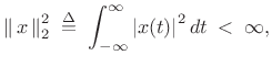
sampled window transform. These spectral samples are illustrated for
a Hamming window transform in Fig.2.3b. Since
, we see that there is one bin per side lobe in the
sampled window transform. These spectral samples are illustrated for
a Hamming window transform in Fig.2.3b. Since ![]() in
Table 5.2, the main lobe is 4 samples wide when critically
sampled. The side lobes are one sample wide, and the samples happen
to hit near some of the side-lobe zero-crossings, which could be
misleading to the untrained eye if only the samples were shown. (Note
that the plot is clipped at -60 dB.)
in
Table 5.2, the main lobe is 4 samples wide when critically
sampled. The side lobes are one sample wide, and the samples happen
to hit near some of the side-lobe zero-crossings, which could be
misleading to the untrained eye if only the samples were shown. (Note
that the plot is clipped at -60 dB.)
![\includegraphics[width=\twidth]{eps/spectsamps}](http://www.dsprelated.com/josimages_new/sasp2/img279.png) |
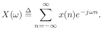
If we now zero pad the Hamming-window by a factor of 2
(append 21 zeros to the length ![]() window and take an
window and take an ![]() point
DFT), we obtain the result shown in Fig.2.4. In this case,
the main lobe is 8 samples wide, and there are two samples per side
lobe. This is significantly better for display even though there is
no new information in the spectrum relative to Fig.2.3.3.10
point
DFT), we obtain the result shown in Fig.2.4. In this case,
the main lobe is 8 samples wide, and there are two samples per side
lobe. This is significantly better for display even though there is
no new information in the spectrum relative to Fig.2.3.3.10
Incidentally, the solid lines in Fig.2.3b and
2.4b indicating the ``true'' DTFT were computed
using a zero-padding factor of
![]() , and they were virtually
indistinguishable visually from
, and they were virtually
indistinguishable visually from ![]() . (
. (![]() is not enough.)
is not enough.)
![\includegraphics[width=\twidth]{eps/spectsamps2}](http://www.dsprelated.com/josimages_new/sasp2/img285.png) |
Zero-Padding for Interpolating Spectral Peaks
For sinusoidal peak-finding, spectral interpolation via zero-padding gets us closer to the true maximum of the main lobe when we simply take the maximum-magnitude FFT-bin as our estimate.
The examples in Fig.2.5 show how zero-padding helps in clarifying the true peak of the sampled window transform. With enough zero-padding, even very simple interpolation methods, such as quadratic polynomial interpolation, will give accurate peak estimates.
![\includegraphics[width=0.7\twidth]{eps/spectsamps3}](http://www.dsprelated.com/josimages_new/sasp2/img286.png) |
Another illustration of zero-padding appears in Section 8.1.3 of [264].
Zero-Phase Zero Padding
The previous zero-padding example used the causal Hamming window, and the appended zeros all went to the right of the window in the FFT input buffer (see Fig.2.4a). When using zero-phase FFT windows (usually the best choice), the zero-padding goes in the middle of the FFT buffer, as we now illustrate.
We look at zero-phase zero-padding using a Blackman window (§3.3.1) which has good, though suboptimal, characteristics for audio work.3.11
Figure 2.6a shows a windowed segment of some sinusoidal data,
with the window also shown as an envelope. Figure 2.6b shows
the same data loaded into an FFT input buffer with a factor of 2
zero-phase zero padding. Note that all time is ``modulo ![]() '' for a
length
'' for a
length ![]() FFT. As a result, negative times
FFT. As a result, negative times ![]() map to
map to ![]() in the
FFT input buffer.
in the
FFT input buffer.
![\includegraphics[width=\twidth]{eps/zpblackmanT}](http://www.dsprelated.com/josimages_new/sasp2/img289.png) |
Figure 2.7a shows the result of performing an FFT on the data
of Fig.2.6b. Since frequency indices are also modulo ![]() ,
the negative-frequency bins appear in the right half of the
buffer. Figure 2.6b shows the same data ``rotated'' so that
bin number is in order of physical frequency from
,
the negative-frequency bins appear in the right half of the
buffer. Figure 2.6b shows the same data ``rotated'' so that
bin number is in order of physical frequency from ![]() to
to ![]() .
If
.
If ![]() is the bin number, then the frequency in Hz is given by
is the bin number, then the frequency in Hz is given by ![]() , where
, where ![]() denotes the sampling rate and
denotes the sampling rate and ![]() is the FFT size.
is the FFT size.
![\includegraphics[width=\twidth]{eps/zpblackmanF}](http://www.dsprelated.com/josimages_new/sasp2/img293.png) |
The Matlab script for creating Figures 2.6 and 2.7 is listed in in §F.1.1.
Matlab/Octave fftshift utility
Matlab and Octave have a simple utility called fftshift that performs this bin rotation. Consider the following example:
octave:4>
fftshift([1 2 3 4])
ans =
  3  4  1  2
octave:5>
If the vector [1 2 3 4] is the output of a length 4 FFT, then the first element (1) is the dc term, and the third element (3) is the point at half the sampling rate (
Another reasonable result would be fftshift([1 2 3 4]) == [4 1
2 3], which defines half the sampling rate as a positive frequency.
However, giving ![]() to the negative frequencies balances giving dc
to the positive frequencies, and the number of samples on both sides
is then the same. For an odd-length DFT, there is no point at
to the negative frequencies balances giving dc
to the positive frequencies, and the number of samples on both sides
is then the same. For an odd-length DFT, there is no point at
![]() , so the result
, so the result
octave:4>
fftshift([1 2 3])
ans =
  3  1  2
octave:5>
is the only reasonable answer, corresponding to frequencies
Index Ranges for Zero-Phase Zero-Padding
Having looked at zero-phase zero-padding ``pictorially'' in matlab
buffers, let's now specify the index-ranges mathematically. Denote
the window length by ![]() (an odd integer) and the FFT length by
(an odd integer) and the FFT length by ![]() (a power of 2). Then the windowed data will occupy indices 0
to
(a power of 2). Then the windowed data will occupy indices 0
to
![]() (positive-time segment), and
(positive-time segment), and ![]() to
to ![]() (negative-time segment). Here we are assuming a 0-based indexing
scheme as used in C or C++. We add 1 to all indices for matlab
indexing to obtain 1:(M-1)/2+1 and N-(M-1)/2+1:N,
respectively. The zero-padding zeros go in between these ranges,
i.e., from
(negative-time segment). Here we are assuming a 0-based indexing
scheme as used in C or C++. We add 1 to all indices for matlab
indexing to obtain 1:(M-1)/2+1 and N-(M-1)/2+1:N,
respectively. The zero-padding zeros go in between these ranges,
i.e., from
![]() to
to
![]() .
.
Summary
To summarize, zero-padding is used for
- padding out to the next higher power of 2 so a Cooley-Tukey FFT can be used with any window length,
- improving the quality of spectral displays, and
- oversampling spectral peaks so that some simple final interpolation will be accurate.
Some examples of interpolated spectral display by means of zero-padding may be seen in §3.4.
Next Section:
Spectrum Analysis Windows
Previous Section:
Introduction and Overview


