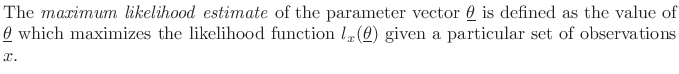
Likelihood Function

Free Books Spectral Audio Signal Processing

The likelihood function $l_x(\underline{\theta})$ is defined as the probability density function of given $\underline{\theta}= [A,\phi,\omega_0 ,\sigma_v^2]^T$ , evaluated at a particular , with $\underline{\theta}$ regarded as a variable.

In other words, the likelihood function $l_x(\underline{\theta})$ is just the PDF of with a particular value of plugged in, and any parameters in the PDF (mean and variance in this case) are treated as variables.

$\textstyle \parbox{0.8\textwidth}{The \emph{maximum likelihood estimate} of the parameter vector $\underline{\theta}$\ is defined as the value of $\underline{\theta}$\ which maximizes the likelihood function $l_x(\underline{\theta})$\ given a particular set of observations $x$.}$

For the sinusoidal parameter estimation problem, given a set of observed data samples , for $n=0,1,2,\ldots,N-1$ , the likelihood function is

$\displaystyle l_x(\underline{\theta}) = \frac{1}{\pi^N \sigma_v^{2N}} e^{-\frac{1}{\sigma_v^2}\sum_{n=0}^{N-1} \left\vert x(n) - {\cal A}e^{j\omega_0 n}\right\vert^2}$

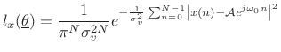(6.50)

and the log likelihood function is

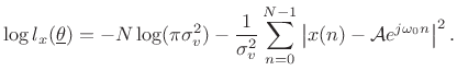$\displaystyle \log l_x(\underline{\theta}) = -N\log(\pi \sigma_v^2) -\frac{1}{\sigma_v^2}\sum_{n=0}^{N-1}\left\vert x(n) - {\cal A}e^{j\omega_0 n}\right\vert^2.$

(6.51)

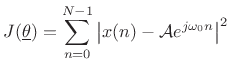We see that the maximum likelihood estimate for the parameters of a sinusoid in Gaussian white noise is the same as the least squares estimate. That is, given $\sigma_v$ , we must find parameters ${\cal A}$ , $\phi$ , and $\omega_0$ which minimize

$\displaystyle J(\underline{\theta}) = \sum_{n=0}^{N-1} \left\vert x(n) - {\cal A}e^{j\omega_0 n}\right\vert^2$

(6.52)

as we saw before in (5.33).

Multiple Sinusoids in Additive Gaussian White Noise

The preceding analysis can be extended to the case of multiple sinusoids in white noise [120]. When the sinusoids are well resolved, i.e., when window-transform side lobes are negligible at the spacings present in the signal, the optimal estimator reduces to finding multiple interpolated peaks in the spectrum.

One exact special case is when the sinusoid frequencies $\omega_k$ coincide with the ``DFT frequencies'' $\omega_k = 2\pi k/N$ , for $k=0,1,2,\ldots,N-1$ . In this special case, each sinusoidal peak sits atop a zero crossing in the window transform associated with every other peak.

To enhance the ``isolation'' among multiple sinusoidal peaks, it is natural to use a window function which minimizes side lobes. However, this is not optimal for short data records since valuable data are ``down-weighted'' in the analysis. Fundamentally, there is a trade-off between peak estimation error due to overlapping side lobes and that due to widening the main lobe. In a practical sinusoidal modeling system, not all sinusoidal peaks are recovered from the data--only the ``loudest'' peaks are measured. Therefore, in such systems, it is reasonable to assure (by choice of window) that the side-lobe level is well below the ``cut-off level'' in dB for the sinusoidal peaks. This prevents side lobes from being comparable in magnitude to sinusoidal peaks, while keeping the main lobes narrow as possible.

When multiple sinusoids are close together such that the associated main lobes overlap, the maximum likelihood estimator calls for a nonlinear optimization. Conceptually, one must search over the possible superpositions of the window transform at various relative amplitudes, phases, and spacings, in order to best ``explain'' the observed data.

Since the number of sinusoids present is usually not known, the number can be estimated by means of hypothesis testing in a Bayesian framework [21]. The ``null hypothesis'' can be ``no sinusoids,'' meaning ``just white noise.''

Non-White Noise

The noise process in (5.44) does not have to be white [120]. In the non-white case, the spectral shape of the noise needs to be estimated and ``divided out'' of the spectrum. That is, a ``pre-whitening filter'' needs to be constructed and applied to the data, so that the noise is made white. Then the previous case can be applied.

Next Section:
Generality of Maximum Likelihood Least Squares
Previous Section:
Maximum Likelihood Sinusoid Estimation