Loudness Spectrogram Examples

We now illustrate a particular Matlab implementation of a loudness spectrogram developed by teaching assistant Patty Huang, following [87,182,88] with slight modifications.^8.9

Multiresolution STFT

Figure 7.4 shows a multiresolution STFT for the same speech signal that was analyzed to produce Fig.7.2. The bandlimits in Hz for the five combined FFTs were , where the last two (in parentheses) were not used due to the signal sampling rate being only kHz. The corresponding window lengths in milliseconds were , where, again, the last two are not needed for this example. Our hop size is chosen to be 1 ms, giving 75% overlap in the highest-frequency channel, and more overlap in lower-frequency channels. Thus, all frequency channels are oversampled along the time dimension. Since many frequency channels from each FFT will be combined via smoothing to form the ``excitation pattern'' (see next section), temporal oversampling is necessary in all channels to avoid uneven weighting of data in the time domain due to the hop size being too large for the shortened effective time-domain windows.

Figure 7.4: Multiresolution Short-Time Fourier Transform (MRSTFT). Compare to the fixed-resolution STFT in Fig.7.2.

Excitation Pattern

Figure 7.5 shows the result of converting the MRSTFT to an excitation pattern [87,182,108]. As mentioned above, this essentially converts the MRSTFT into a better approximation of an auditory filter bank by non-uniformly resampling the frequency axis using auditory interpolation kernels.

Note that the harmonics are now clearly visible only up to approximately 20 ERBs, and only the first four or five harmonics are visible during voiced segments. During voiced segments, the formant structure is especially clearly visible at about 25 ERBs. Also note that ``pitch pulses'' are visible as very thin, alternating, dark and light vertical stripes above 25 ERBs or so; the dark lines occur just after glottal closure, when the voiced-speech period has a strong peak in the time domain.

Figure 7.5: Excitation pattern versus time, computed from the MRSTFT.

Nonuniform Spectral Resampling

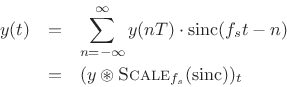
Recall sinc interpolation of a discrete-time signal [270]:

And recall asinc interpolation of a sampled spectrum (§2.5.2):

We see that resampling consists of an inner-product between the given samples with a continuous interpolation kernel that is sampled where needed to satisfy the needs of the inner product operation. In the time domain, our interpolation kernel is a scaled sinc function, while in the frequency domain, it is an asinc function. The interpolation kernel can of course be horizontally scaled to alter bandwidth [270], or more generally reshaped to introduce a more general windowing in the opposite domain:

• Width of interpolation kernel (main-lobe width) 1/width-in-other-domain

• Shape of interpolation kernel gain profile (window) in other domain

Getting back to non-uniform resampling of audio spectra, we have that an auditory-filter frequency-response can be regarded as a frequency-dependent interpolation kernel for nonuniformly resampling the STFT frequency axis. In other words, an auditory filter bank may be implemented as a non-uniform resampling of the uniformly sampled frequency axis provided by an ordinary FFT, using the auditory filter shape as the interpolation kernel.

When the auditory filters vary systematically with frequency, there may be an equivalent non-uniform frequency-warping followed by a uniform sampling of the (warped) frequency axis. Thus, an alternative implementation of an auditory filter bank is to apply an FFT (implementing a uniform filter bank) to a signal having a properly prewarped spectrum, where the warping is designed to approximate whatever auditory frequency axis is desired. This approach is discussed further in Appendix E. (See also §2.5.2.)

Auditory Filter Shapes

The topic of auditory filter banks was introduced in §7.3.1 above. In this implementation, the auditory filters were synthesized from the Equivalent Rectangular Bandwidth (ERB) frequency scale, discussed in §E.5. The auditory filter-bank shapes are a function of level, so, ideally, the true physical amplitude level of the input signal at the ear(s) should be known. The auditory filter shape at 1 kHz in response to a sinusoidal excitation for a variety of amplitudes is shown in Fig.7.6.

Figure 7.6: Excitation patterns for a 1 kHz sinusoid at different levels.

Specific Loudness

Figure 7.7 shows the specific loudness computed from the excitation pattern of Fig.7.5. As mentioned above, it is a compressive nonlinearity that depends on level and also frequency.

Figure 7.7: Specific loudness computed from the excitation pattern each time step.

Spectrograms Compared

Figure 7.8 shows all four previous spectrogram figures in a two-by-two matrix for ease of cross-reference.

Figure 7.8: (a) Classic spectrogram. (b) Multiresolution STFT dB magnitude. (c) Excitation pattern. (d) Specific loudness.

Instantaneous, Short-Term, and Long-Term Loudness

Finally, Fig.7.9 shows the instantaneous loudness, short-term loudness, and long-term loudness functions overlaid, for the same speech sample used in the previous plots. These are all single-valued functions of time which indicate the relative loudness of the signal on different time scales. See [88] for further discussion. While the lower plot looks reasonable, the upper plot (in sones) predicts only three audible time regions. Evidently, it corresponds to a very low listening level.^8.10

The instantaneous loudness is simply the sum of the specific loudness over all frequencies. The short- and long-term loudnesses are derived by smoothing the instantaneous loudness with respect to time using various psychoacoustically motivated time constants [88]. The smoothing is nonlinear because the loudness tracks a rising amplitude very quickly, while decaying with a slower time constant.^8.11 The loudness of a brief sound is taken to be the local maximum of the short-term loudness curve. The long-term loudness is related to loudness memory over time.

The upper plot gives loudness in sones, which is based on loudness perception experiments [276]; at 1 kHz and above, loudness perception is approximately logarithmic above 50 dB SPL or so, while below that, it tends toward being more linear. The lower plot is given in phons, which is simply sound pressure level (SPL) in dB at 1 kHz [276, p. 111]; at other frequencies, the amplitude in phons is defined by following an ``equal-loudness curve'' over to 1 kHz and reading off the level there in dB SPL. This means, e.g., that all pure tones have the same perceived loudness when they are at the same phon level, and the dB SPL at 1 kHz defines the loudness of such tones in phons.

Figure 7.9: Total instantaneous, short-term, and long-term loudness, computed from the specific loudness. Top: sone loudness scale. Bottom: loudness in phons.

Sign in