


Optimal FIR Digital Filter Design
We now look briefly at the topic of optimal FIR filter design. We saw examples above of optimal Chebyshev designs (§4.5.2). and an oversimplified optimal least-squares design (§4.3). Here we elaborate a bit on optimality formulations under various error norms.
Lp norms
The ![]() norm of an
norm of an ![]() -dimensional vector (signal)
-dimensional vector (signal) ![]() is defined as
is defined as
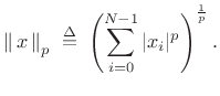 |
(5.27) |
Special Cases
 norm
norm

(5.28)
- Sum of the absolute values of the elements
- ``City block'' distance
 norm
norm
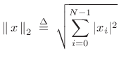
(5.29)
- ``Euclidean'' distance
- Minimized by ``Least Squares'' techniques
-
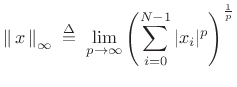
 norm
norm
In the limit as
 , the
, the  norm of
  is dominated by the maximum element of
. Optimal Chebyshev
filters minimize this norm of the frequency-response error.
is dominated by the maximum element of
. Optimal Chebyshev
filters minimize this norm of the frequency-response error.
Filter Design using Lp Norms
Formulated as an ![]() norm minimization, the FIR filter design problem
can be stated as follows:
norm minimization, the FIR filter design problem
can be stated as follows:
| (5.31) |
where
 FIR filter coefficients
-
 suitable discrete set of frequencies
-
 desired (complex) frequency response
-
 obtained frequency response (typically fft(h))
-
 (optional) error weighting function
Optimal Chebyshev FIR Filters
As we've seen above, the defining characteristic of FIR filters
optimal in the Chebyshev sense is that they minimize the maximum
frequency-response error-magnitude over the frequency axis. In
other terms, an optimal Chebyshev FIR filter is optimal in the
minimax sense: The filter coefficients are chosen to minimize
the worst-case error (maximum weighted error-magnitude ripple)
over all frequencies. This also means it is optimal in the
![]() sense because, as noted above, the
sense because, as noted above, the
![]() norm of a weighted
frequency-response error
norm of a weighted
frequency-response error
![]() is the maximum magnitude over all frequencies:
is the maximum magnitude over all frequencies:
| (5.32) |
Thus, we can say that an optimal Chebyshev filter minimizes the
The optimal Chebyshev FIR filter can often be found effectively using the Remez multiple exchange algorithm (typically called the Parks-McClellan algorithm when applied to FIR filter design) [176,224,66]. This was illustrated in §4.6.4 above. The Parks-McClellan/Remez algorithm also appears to be the most efficient known method for designing optimal Chebyshev FIR filters (as compared with, say linear programming methods using matlab's linprog as in §3.13). This algorithm is available in Matlab's Signal Processing Toolbox as firpm() (remez() in (Linux) Octave).5.13There is also a version of the Remez exchange algorithm for complex FIR filters. See §4.10.7 below for a few details.
The Remez multiple exchange algorithm has its limitations, however. In particular, convergence of the FIR filter coefficients is unlikely for FIR filters longer than a few hundred taps or so.
Optimal Chebyshev FIR filters are normally designed to be linear
phase [263] so that the desired frequency response
![]() can be taken to be real (i.e., first a zero-phase
FIR filter is designed). The design of linear-phase FIR filters in
the frequency domain can therefore be characterized as real
polynomial approximation on the unit circle [229,258].
can be taken to be real (i.e., first a zero-phase
FIR filter is designed). The design of linear-phase FIR filters in
the frequency domain can therefore be characterized as real
polynomial approximation on the unit circle [229,258].
In optimal Chebyshev filter designs, the error exhibits an
equiripple characteristic--that is, if the desired
response is ![]() and the ripple magnitude is
and the ripple magnitude is ![]() , then
the frequency response of the optimal FIR filter (in the unweighted
case, i.e.,
, then
the frequency response of the optimal FIR filter (in the unweighted
case, i.e.,
![]() for all
for all ![]() ) will oscillate between
) will oscillate between
![]() and
and
![]() as
as ![]() increases.
The powerful alternation theorem characterizes optimal
Chebyshev solutions in terms of the alternating error peaks.
Essentially, if one finds sufficiently many for the given FIR filter
order, then you have found the unique optimal Chebyshev solution
[224]. Another remarkable result is that the Remez
multiple exchange converges monotonically to the unique optimal
Chebyshev solution (in the absence of numerical round-off errors).
increases.
The powerful alternation theorem characterizes optimal
Chebyshev solutions in terms of the alternating error peaks.
Essentially, if one finds sufficiently many for the given FIR filter
order, then you have found the unique optimal Chebyshev solution
[224]. Another remarkable result is that the Remez
multiple exchange converges monotonically to the unique optimal
Chebyshev solution (in the absence of numerical round-off errors).
Fine online introductions to the theory and practice of Chebyshev-optimal FIR filter design are given in [32,283].
The window method (§4.5) and Remez-exchange method together span many practical FIR filter design needs, from ``quick and dirty'' to essentially ideal FIR filters (in terms of conventional specifications).
Least-Squares Linear-Phase FIR Filter Design
Another versatile, effective, and often-used case is the weighted least squares method, which is implemented in the matlab function firls and others. A good general reference in this area is [204].
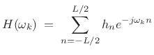
Let the FIR filter length be ![]() samples, with
samples, with ![]() even, and suppose
we'll initially design it to be centered about the time origin (``zero
phase''). Then the frequency response is given on our frequency grid
even, and suppose
we'll initially design it to be centered about the time origin (``zero
phase''). Then the frequency response is given on our frequency grid
![]() by
by
 |
(5.33) |
Enforcing even symmetry in the impulse response, i.e.,
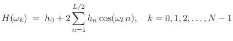 |
(5.34) |
or, in matrix form:
![$\displaystyle \underbrace{\left[ \begin{array}{c} H(\omega_0) \\ H(\omega_1) \\ \vdots \\ H(\omega_{N-1}) \end{array} \right]}_{{\underline{d}}} = \underbrace{\left[ \begin{array}{ccccc} 1 & 2\cos(\omega_0) & \dots & 2\cos[\omega_0(L/2)] \\ 1 & 2\cos(\omega_1) & \dots & 2\cos[\omega_1(L/2)] \\ \vdots & \vdots & & \vdots \\ 1 & 2\cos(\omega_{N-1}) & \dots & 2\cos[\omega_{N-1}(L/2)] \end{array} \right]}_\mathbf{A} \underbrace{\left[ \begin{array}{c} h_0 \\ h_1 \\ \vdots \\ h_{L/2} \end{array} \right]}_{{\underline{h}}} \protect$](http://www.dsprelated.com/josimages_new/sasp2/img849.png)
Recall from §3.13.8, that the Remez multiple exchange
algorithm is based on this formulation internally. In that case, the
left-hand-side includes the alternating error, and the frequency grid
![]() iteratively seeks the frequencies of maximum error--the
so-called extremal frequencies.
iteratively seeks the frequencies of maximum error--the
so-called extremal frequencies.
In matrix notation, our filter-design problem can be stated as (cf. §3.13.8)
| (5.36) |
where these quantities are defined in (4.35). We can denote the optimal least-squares solution by
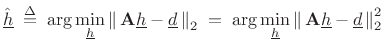 |
(5.37) |
To find
This is a quadratic form in
| (5.39) |
with solution
![$\displaystyle \zbox {{\underline{\hat{h}}}\eqsp \left[(\mathbf{A}^T\mathbf{A})^{-1}\mathbf{A}^T\right]{\underline{d}}.}$](http://www.dsprelated.com/josimages_new/sasp2/img859.png) |
(5.40) |
The matrix
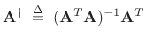 |
(5.41) |
is known as the (Moore-Penrose) pseudo-inverse of the matrix
Geometric Interpretation of Least Squares
Typically, the number of frequency constraints is much greater than the number of design variables (filter coefficients). In these cases, we have an overdetermined system of equations (more equations than unknowns). Therefore, we cannot generally satisfy all the equations, and are left with minimizing some error criterion to find the ``optimal compromise'' solution.
In the case of least-squares approximation, we are minimizing the Euclidean distance, which suggests the geometrical interpretation shown in Fig.4.19.
![\begin{psfrags}
% latex2html id marker 14494\psfrag{Ax}{{\Large $\mathbf{A}{\underline{\hat{h}}}$}}\psfrag{b}{{\Large ${\underline{d}}$}}\psfrag{column}{{\Large column-space of $\mathbf{A}$}}\psfrag{space}{}\begin{figure}[htbp]
\includegraphics[width=3in]{eps/lsq}
\caption{Geometric interpretation of orthogonal
projection of the vector ${\underline{d}}$\ onto the column-space of $\mathbf{A}$.}
\end{figure}
\end{psfrags}](http://www.dsprelated.com/josimages_new/sasp2/img862.png)
Thus, the desired vector
![]() is the vector sum of its
best least-squares approximation
is the vector sum of its
best least-squares approximation
![]() plus an orthogonal error
plus an orthogonal error ![]() :
:
| (5.42) |
In practice, the least-squares solution
| (5.43) |
Figure 4.19 suggests that the error vector
| (5.44) |
This is how the orthogonality principle can be used to derive the fact that the best least squares solution is given by
| (5.45) |
In matlab, it is numerically superior to use ``h= A
We will return to least-squares optimality in §5.7.1 for the purpose of estimating the parameters of sinusoidal peaks in spectra.
Matlab Support for Least-Squares FIR Filter Design
Some of the available functions are as follows:
- firls - least-squares linear-phase FIR filter design
for piecewise constant desired amplitude responses -- also designs
Hilbert transformers and differentiators
- fircls - constrained least-squares linear-phase FIR
filter design for piecewise constant desired amplitude responses --
constraints provide lower and upper bounds on the frequency response
- fircls1 - constrained least-squares linear-phase FIR
filter design for lowpass and highpass filters -- supports relative
weighting of pass-band and stop-band error
For more information, type help firls and/or doc firls, etc., and refer to the ``See Also'' section of the documentation for pointers to more relevant functions.
Chebyshev FIR Design via Linear Programming
We return now to the
![]() -norm minimization problem of §4.10.2:
-norm minimization problem of §4.10.2:
and discuss its formulation as a linear programming problem, very similar to the optimal window formulations in §3.13. We can rewrite (4.46) as
| (5.47) |
where
| s.t. | (5.48) |
Introducing a new variable
![$\displaystyle \tilde{{\underline{h}}} \isdefs \left[ \begin{array}{c} {\underline{h}}\\ t \end{array} \right],$](http://www.dsprelated.com/josimages_new/sasp2/img876.png) |
(5.49) |
then we can write
![$\displaystyle t \eqsp f^T \tilde{{\underline{h}}} \isdefs \left[\begin{array}{cccc} 0 & \cdots & 0 & 1 \end{array}\right] \tilde{{\underline{h}}},$](http://www.dsprelated.com/josimages_new/sasp2/img877.png) |
(5.50) |
and our optimization problem can be written in more standard form:
| s.t. | ![$\displaystyle \left\vert [\begin{array}{cc} a_k^T \; 0\\ \end{array} ] \cdot \tilde{{\underline{h}}} -{\underline{d}}_k \right\vert
\;<\; \tilde{{\underline{h}}}^T f^T\tilde{{\underline{h}}}$](http://www.dsprelated.com/josimages_new/sasp2/img880.png) |
(5.51) |
Thus, we are minimizing a linear objective, subject to a set of linear inequality constraints. This is known as a linear programming problem, as discussed previously in §3.13.1, and it may be solved using the matlab linprog function. As in the case of optimal window design, linprog is not normally as efficient as the Remez multiple exchange algorithm (firpm), but it is more general, allowing for linear equality and inequality constraints to be imposed.
More General Real FIR Filters
So far we have looked at the design of linear phase filters. In this
case,
![]() ,
,
![]() and
and
![]() are all real. In some
applications, we need to specify both the magnitude and
phase of the frequency response. Examples include
are all real. In some
applications, we need to specify both the magnitude and
phase of the frequency response. Examples include
- minimum phase filters [263],
- inverse filters (``deconvolution''),
- fractional delay filters [266],
- interpolation polyphase subfilters (Chapter 11)
Nonlinear-Phase FIR Filter Design
Above, we considered only linear-phase (symmetric) FIR filters. The same methods also work for antisymmetric FIR filters having a purely imaginary frequency response, when zero-centered, such as differentiators and Hilbert transformers [224].
We now look at extension to nonlinear-phase FIR filters,
managed by treating the real and imaginary parts separately in the
frequency domain [218]. In the
nonlinear-phase case, the frequency response is complex in
general. Therefore, in the formulation Eq.![]() (4.35) both
(4.35) both
![]() and
and
![]() are complex, but we still desire the FIR filter coefficients
are complex, but we still desire the FIR filter coefficients
![]() to be real. If we try to use '
to be real. If we try to use '
![]() ' or pinv in
matlab, we will generally get a complex result for
' or pinv in
matlab, we will generally get a complex result for
![]() .
.
Problem Formulation
| (5.52) |
where
| (5.53) |
which can be written as
| (5.54) |
or
![$\displaystyle \min_{\underline{h}}\left\vert \left\vert \left[ \begin{array}{c} {\cal{R}}(\mathbf{A}) \\ {\cal{I}}(\mathbf{A}) \end{array} \right] {\underline{h}} - \left[ \begin{array}{c} {\cal{R}}({\underline{d}}) \\ {\cal{I}}({\underline{d}}) \end{array}\right] \right\vert \right\vert _2^2$](http://www.dsprelated.com/josimages_new/sasp2/img887.png) |
(5.55) |
which is written in terms of only real variables.
In summary, we can use the standard least-squares solvers in matlab and end up with a real solution for the case of complex desired spectra and nonlinear-phase FIR filters.
Matlab for General FIR Filter Design
The cfirpm function (formerly cremez)
[116,117] in the Matlab Signal
Processing Toolbox performs complex
![]() FIR filter design
(``Complex FIR Parks-McClellan''). Convergence is theoretically
guaranteed for arbitrary magnitude and phase specifications
versus frequency. It reduces to Parks-McClellan algorithm (Remez
second algorithm) as a special case.
FIR filter design
(``Complex FIR Parks-McClellan''). Convergence is theoretically
guaranteed for arbitrary magnitude and phase specifications
versus frequency. It reduces to Parks-McClellan algorithm (Remez
second algorithm) as a special case.
The firgr function (formerly gremez) in the Matlab
Filter Design Toolbox performs ``generalized''
![]() FIR filter
design, adding support for minimum-phase FIR filter design, among
other features [254].
FIR filter
design, adding support for minimum-phase FIR filter design, among
other features [254].
Finally, the fircband function in the Matlab DSP System Toolbox designs a variety of real FIR filters with various filter-types and constraints supported.
This is of course only a small sampling of what is available. See, e.g., the Matlab documentation on its various toolboxes relevant to filter design (especially the Signal Processing and Filter Design toolboxes) for much more.
Second-Order Cone Problems
In Second-Order Cone Problems (SOCP), a linear function is minimized over the intersection of an affine set and the product of second-order (quadratic) cones [153,22]. Nonlinear, convex problem including linear and (convex) quadratic programs are special cases. SOCP problems are solved by efficient primal-dual interior-point methods. The number of iterations required to solve a problem grows at most as the square root of the problem size. A typical number of iterations ranges between 5 and 50, almost independent of the problem size.
Resources
- LIPSOL: Matlab code for linear programming using interior point methods.
- Matlab's linprog (in the Optimization Toolbox)
- Octave's lp (SourceForge package)
Nonlinear Optimization in Matlab
There are various matlab functions available for nonlinear optimizations as well. These can be utilized in more exotic FIR filter designs, such as designs driven more by perceptual criteria:
- The fsolve function in Octave, or the Matlab Optimization Toolbox, attempts to solve unconstrained, overdetermined, nonlinear systems of equations.
- The Octave function sqp handles constrained nonlinear optimization.
- The Octave optim package includes many additional functions such as leasqr for performing Levenberg-Marquardt nonlinear regression. (Say, e.g., which leasqr and explore its directory.)
- The Matlab Optimization Toolbox similarly contains many functions for optimization.
Next Section:
Spectrum of a Sinusoid
Previous Section:
Minimum-Phase and Causal Cepstra


