


Polyphase Decomposition
The previous section derived an efficient polyphase implementation of
an FIR filter ![]() whose output was downsampled by the factor
whose output was downsampled by the factor ![]() . The
derivation was based on commuting the downsampler with the FIR
summer. We now derive the polyphase representation of a filter of any
length algebraically by splitting the impulse response
. The
derivation was based on commuting the downsampler with the FIR
summer. We now derive the polyphase representation of a filter of any
length algebraically by splitting the impulse response ![]() into
into
![]() polyphase components.
polyphase components.
Two-Channel Case
The simplest nontrivial case is ![]() channels. Starting with a
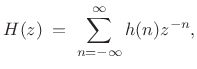
general linear time-invariant filter
channels. Starting with a
general linear time-invariant filter
 |
(12.6) |
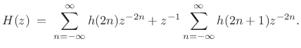
we may separate the even- and odd-indexed terms to get
 |
(12.7) |
We define the polyphase component filters as follows:
![\begin{eqnarray*}
E_0(z)&=&\sum_{n=-\infty}^{\infty}h(2n)z^{-n}\\ [5pt]
E_1(z)&=&\sum_{n=-\infty}^{\infty}h(2n+1)z^{-n}
\end{eqnarray*}](http://www.dsprelated.com/josimages_new/sasp2/img1958.png)
![]() and
and ![]() are the polyphase components
of the polyphase decomposition of
are the polyphase components
of the polyphase decomposition of ![]() for
for ![]() .
.
Now write ![]() in terms of its polyphase components:
in terms of its polyphase components:
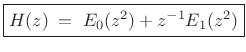 |
(12.8) |
As a simple example, consider
| (12.9) |
Then the polyphase component filters are
![\begin{eqnarray*}
E_0(z) &=& 1 + 3z^{-1}\\ [5pt]
E_1(z) &=& 2 + 4z^{-1}
\end{eqnarray*}](http://www.dsprelated.com/josimages_new/sasp2/img1963.png)
and
| (12.10) |
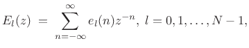
N-Channel Polyphase Decomposition
![\includegraphics[scale=0.8]{eps/polytime}](http://www.dsprelated.com/josimages_new/sasp2/img1965.png)
For the general case of arbitrary ![]() , the basic idea is to decompose
, the basic idea is to decompose
![]() into its periodically interleaved subsequences, as indicated
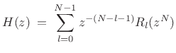
schematically in Fig.11.9. The polyphase decomposition into
into its periodically interleaved subsequences, as indicated
schematically in Fig.11.9. The polyphase decomposition into
![]() channels is given by
channels is given by
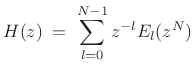
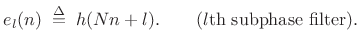
where the subphase filters are defined by
 |
(12.12) |
with
 |
(12.13) |
The signal
![\begin{psfrags}
% latex2html id marker 29755\psfrag{M}{{\normalsize $N$}}\psfrag{ztl}{{\Large $z^l$}}\psfrag{h[n]}{{\Large $h(n)$}}\psfrag{eln}{{\Large $e_l(n)$}}\begin{figure}[htbp]
\includegraphics[width=0.5\twidth]{eps/polypick}
\caption{Advance by $l$\ samples followed by a downsampling by the factor $N$.}
\end{figure}
\end{psfrags}](http://www.dsprelated.com/josimages_new/sasp2/img1970.png)
Type II Polyphase Decomposition
The polyphase decomposition of ![]() into
into ![]() channels in
(11.11) may be termed a ``type I'' polyphase decomposition. In
the ``type II'', or reverse polyphase decomposition, the powers
of
channels in
(11.11) may be termed a ``type I'' polyphase decomposition. In
the ``type II'', or reverse polyphase decomposition, the powers
of ![]() progress in the opposite direction:
progress in the opposite direction:
 |
(12.14) |
We will see that we need type I for analysis filter banks and type II for synthesis filter banks in a general ``perfect reconstruction filter bank'' analysis/synthesis system.
Filtering and Downsampling, Revisited
Let's return to the example of §11.1.3, but
this time have the FIR lowpass filter h(n) be length ![]() ,
,
![]() . In this case, the
. In this case, the ![]() polyphase filters,
polyphase filters, ![]() , are
each length
, are
each length ![]() .12.2 Recall that
.12.2 Recall that
| (12.15) |
leading to the result shown in Fig.11.11.
![\includegraphics[width=0.7\twidth]{eps/down_FIR_poly}](http://www.dsprelated.com/josimages_new/sasp2/img1974.png)
![\includegraphics[width=0.7\twidth]{eps/down_FIR_poly_com}](http://www.dsprelated.com/josimages_new/sasp2/img1975.png)
Next, we commute the ![]() :
:![]() downsampler through the adders and
upsampled (stretched) polyphase filters
downsampler through the adders and
upsampled (stretched) polyphase filters ![]() to obtain
Fig.11.12. Commuting the downsampler through the
subphase filters
to obtain
Fig.11.12. Commuting the downsampler through the
subphase filters ![]() to obtain
to obtain ![]() is an example of a
multirate noble identity.
is an example of a
multirate noble identity.
Multirate Noble Identities
Figure 11.13 illustrates the so-called noble identities for
commuting downsamplers/upsamplers with ``sparse transfer functions''
that can be expressed a function of ![]() . Note that downsamplers
and upsamplers are linear, time-varying operators. Therefore,
operation order is important. Also note that adders and multipliers
(any memoryless operators) may be commuted across downsamplers and
upsamplers, as shown in Fig.11.14.
. Note that downsamplers
and upsamplers are linear, time-varying operators. Therefore,
operation order is important. Also note that adders and multipliers
(any memoryless operators) may be commuted across downsamplers and
upsamplers, as shown in Fig.11.14.
![\begin{psfrags}
% latex2html id marker 29805\psfrag{nd}{ $N\downarrow$\ }\psfrag{hz}{ $H(z)$\ }\psfrag{hzn}{ $H(z^N)$\ }\psfrag{equal}{ $\equiv$\ }\begin{figure}[htbp]
\includegraphics[width=0.9\twidth]{eps/noble}
\caption{Multirate noble identities}
\end{figure} % was 6in
\end{psfrags}](http://www.dsprelated.com/josimages_new/sasp2/img1979.png)
![\includegraphics[width=0.9\twidth]{eps/noble_commute}](http://www.dsprelated.com/josimages_new/sasp2/img1980.png)
Next Section:
Critically Sampled Perfect Reconstruction Filter Banks
Previous Section:
Upsampling and Downsampling


