


Processing Gain
A basic property of noise signals is that they add non-coherently. This means they sum on a
power basis instead of an amplitude basis. Thus, for
example, if you add two separate realizations of a random process
together, the total energy rises by approximately 3 dB
(
![]() ). In contrast to this, sinusoids and other
deterministic signals can add coherently. For example, at the midpoint between two
loudspeakers putting out identical signals, a sinusoidal signal is
). In contrast to this, sinusoids and other
deterministic signals can add coherently. For example, at the midpoint between two
loudspeakers putting out identical signals, a sinusoidal signal is ![]() dB louder than the signal out of each loudspeaker alone (cf.
dB louder than the signal out of each loudspeaker alone (cf. ![]() dB
for uncorrelated noise).
dB
for uncorrelated noise).
Coherent addition of sinusoids and noncoherent addition of noise can be used to obtain any desired signal to noise ratio in a spectrum analysis of sinusoids in noise. Specifically, for each doubling of the periodogram block size in Welch's method, the signal to noise ratio (SNR) increases by 3 dB (6 dB spectral amplitude increase for all sinusoids, minus 3 dB increase for the noise spectrum).
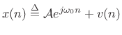
Consider a single complex sinusoid in white noise as introduced in (5.32):
 |
(7.39) |
where
![\begin{eqnarray*}
X(\omega_k)
&=& \hbox{\sc DFT}_k(x) = \sum_{n=0}^{N-1}\left[{\cal A}e^{j\omega_0 n} + v(n)\right] e^{-j\omega_k n}\\
&=& {\cal A}\sum_{n=0}^{N-1}e^{j(\omega_0 -\omega_k) n} + \sum_{n=0}^{N-1}v(n) e^{-j\omega_k n}\\
&=& {\cal A}\frac{1-e^{j(\omega_0 -\omega_k)N}}{1-e^{j(\omega_0 -\omega_k)}} + V_N(\omega_k)\\
\end{eqnarray*}](http://www.dsprelated.com/josimages_new/sasp2/img1214.png)
For simplicity, let
![]() for some
for some ![]() . That is, suppose for
now that
. That is, suppose for
now that ![]() is one of the DFT frequencies
is one of the DFT frequencies ![]() ,
,
![]() .
Then
.
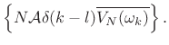
Then
![\begin{eqnarray*}
X(\omega_k) &=& \left\{\begin{array}{ll}
N{\cal A}+V_N(\omega_k), & k=l \\ [5pt]
V_N(\omega_k), & k\neq l \\
\end{array} \right.\\
&=& N{\cal A}\delta(k-l)+V_N(\omega_k)
\end{eqnarray*}](http://www.dsprelated.com/josimages_new/sasp2/img1218.png)
for
![]() . Squaring the absolute value gives
. Squaring the absolute value gives
 |
(7.40) |
Since
| (7.41) |
where
The final term can be expanded as
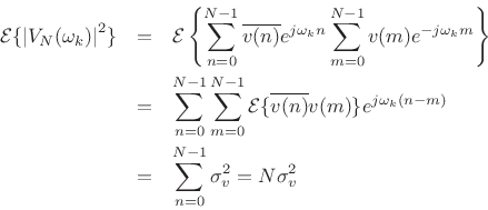
since
![]() because
because ![]() is white noise.
is white noise.
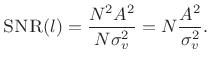
In conclusion, we have derived that the average squared-magnitude DFT
of ![]() samples of a sinusoid in white noise is given by
samples of a sinusoid in white noise is given by
| (7.42) |
where
 |
(7.43) |
In the time domain, the mean square for the signal is
Another way of viewing processing gain is to consider that the DFT
performs a change of coordinates on the observations ![]() such
that all of the signal energy ``piles up'' in one coordinate
such
that all of the signal energy ``piles up'' in one coordinate
![]() , while the noise energy remains uniformly distributed
among all of the coordinates.
, while the noise energy remains uniformly distributed
among all of the coordinates.
A practical implication of the above discussion is that it is
meaningless to quote signal-to-noise ratio in the frequency domain
without reporting the relevant bandwidth. In the above example, the
SNR could be reported as
![]() in band
in band ![]() .
.
The above analysis also makes clear the effect of bandpass
filtering on the signal-to-noise ratio (SNR). For example, consider a dc level
![]() in white noise with variance
in white noise with variance
![]() . Then the SNR
(mean-square level ratio) in the time domain is
. Then the SNR
(mean-square level ratio) in the time domain is
![]() .
Low-pass filtering at
.
Low-pass filtering at
![]() cuts the noise energy in half but
leaves the dc component unaffected, thereby increasing the SNR by
cuts the noise energy in half but
leaves the dc component unaffected, thereby increasing the SNR by
![]() dB. Each halving of the lowpass cut-off
frequency adds another 3 dB to the SNR. Since the signal is a dc
component (zero bandwidth), this process can be repeated indefinitely
to achieve any desired SNR. The narrower the lowpass filter, the
higher the SNR. Similarly, for sinusoids, the narrower the bandpass
filter centered on the sinusoid's frequency, the higher the SNR.
dB. Each halving of the lowpass cut-off
frequency adds another 3 dB to the SNR. Since the signal is a dc
component (zero bandwidth), this process can be repeated indefinitely
to achieve any desired SNR. The narrower the lowpass filter, the
higher the SNR. Similarly, for sinusoids, the narrower the bandpass
filter centered on the sinusoid's frequency, the higher the SNR.
Next Section:
The Panning Problem
Previous Section:
Filtered White Noise


