


The Short-Time Fourier Transform
The Short-Time Fourier Transform (STFT) (or short-term Fourier transform) is a powerful general-purpose tool for audio signal processing [7,9,8]. It defines a particularly useful class of time-frequency distributions [43] which specify complex amplitude versus time and frequency for any signal. We are primarily concerned here with tuning the STFT parameters for the following applications:
- Approximating the time-frequency analysis performed by the ear for purposes of spectral display.
- Measuring model parameters in a short-time spectrum.
Examples of the second case include estimating the decay-time-versus-frequency for vibrating strings [288] and body resonances [119], or measuring as precisely as possible the fundamental frequency of a periodic signal [106] based on tracking its many harmonics in the STFT [64].
An interesting example for which cases 1 and 2 normally coincide is pitch detection (case 1) and fundamental frequency estimation (case 2). Here, ``fundamental frequency'' is defined as the lowest frequency present in a series of harmonic overtones, while ``pitch'' is defined as the perceived fundamental frequency; perceived pitch can be measured, for example, by comparing to a harmonic reference tone such as a sawtooth waveform. (Thus, by definition, the pitch of a sawtooth waveform is its fundamental frequency.) When harmonics are stretched so that they become slightly inharmonic, pitch perception corresponds to a (possibly non-existent) compromise fundamental frequency, the harmonics of which ``best fit'' the most audible overtones in some sense. The topic of ``pitch detection'' in the signal processing literature is often really about fundamental frequency estimation [106], and this distinction is lost. This is not a problem for strictly periodic signals.
Mathematical Definition of the STFT
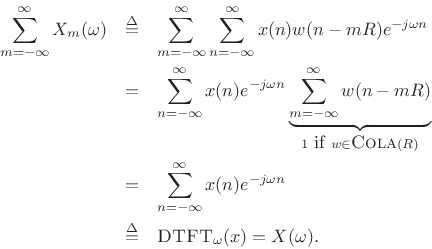
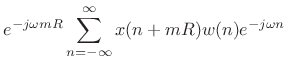
The usual mathematical definition of the STFT is
[9]
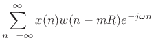
where

If the window ![]() has the
Constant OverLap-Add (COLA) property at hop-size
has the
Constant OverLap-Add (COLA) property at hop-size ![]() , i.e., if
, i.e., if
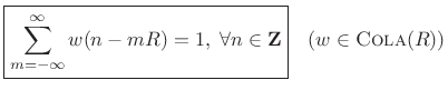
then the sum of the successive DTFTs over time equals the DTFT of the whole signal
We will say that windows satisfying
![]() (or some
constant) for all
(or some
constant) for all
![]() are said to be
are said to be
![]() . For example,
the length
. For example,
the length ![]() rectangular window is clearly
rectangular window is clearly
![]() (no overlap).
The Bartlett window and all windows in the generalized Hamming family
(Chapter 3) are
(no overlap).
The Bartlett window and all windows in the generalized Hamming family
(Chapter 3) are
![]() (50% overlap),
when the endpoints are handled correctly.8.1 A
(50% overlap),
when the endpoints are handled correctly.8.1 A
![]() example
is depicted in
Fig.8.9. Any window that is
example
is depicted in
Fig.8.9. Any window that is
![]() is also
is also
![]() ,
for
,
for
![]() , provided
, provided ![]() is an
integer.8.2 We will explore COLA windows
more completely in Chapter 8.
is an
integer.8.2 We will explore COLA windows
more completely in Chapter 8.
When using the short-time Fourier transform for signal processing, as taken up in Chapter 8, the COLA requirement is important for avoiding artifacts. For usage as a spectrum analyzer for measurement and display, the COLA requirement can often be relaxed, as doing so only means we are not weighting all information equally in our analysis. Nothing disastrous happens, for example, if we use 50% overlap with the Blackman window in a short-time spectrum analysis over time--the results look fine; however, in such a case, data falling near the edges of the window will have a slightly muted impact on the results relative to data falling near the window center, because the Blackman window is not COLA at 50% overlap.
Practical Computation of the STFT
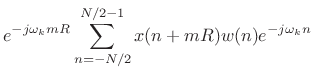
While the definition of the STFT in (7.1) is useful for theoretical work, it is not really a specification of a practical STFT. In practice, the STFT is computed as a succession of FFTs of windowed data frames, where the window ``slides'' or ``hops'' forward through time. We now derive such an implementation of the STFT from its mathematical definition.
The STFT in (7.1) can be rewritten, adding ![]() to
to ![]() , as
, as
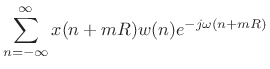
In this form, the data centered about time
Since indexing in the DFT is modulo
Summary of STFT Computation Using FFTs
- Read
 samples of the input signal
  into a local buffer of
length
into a local buffer of
length  which is initially zeroed
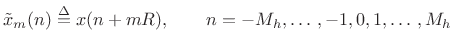
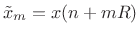
We call the
the  th frame of the input signal, and
 the
th time normalized input frame
(time-normalized by translating it to time zero). The frame length is
the
th time normalized input frame
(time-normalized by translating it to time zero). The frame length is
 , which we assume to be odd for reasons to be
discussed later. The time advance
, which we assume to be odd for reasons to be
discussed later. The time advance  (in samples) from one frame to
the next is called the
hop size
or
step size.
(in samples) from one frame to
the next is called the
hop size
or
step size.
- Multiply the data frame pointwise by a length
spectrum
analysis window
 to obtain the
th
windowed data frame (time normalized):
to obtain the
th
windowed data frame (time normalized):
- Extend
 with zeros on both sides to obtain a
zero-padded frame:
with zeros on both sides to obtain a
zero-padded frame:
![$\displaystyle \tilde{x}_m^{w,z}(n) \isdef \left\{\begin{array}{ll} \tilde{x}_m^w(n), & \left\vert n\right\vert\leq M_h\isdef {\frac{M-1}{2}} \\ [5pt] 0, & M_h< n \leq {\frac{N}{2}}-1 \\ [5pt] 0, & -{\frac{N}{2}}\leq n < -M_h \\ \end{array} \right.$](http://www.dsprelated.com/josimages_new/sasp2/img1274.png)
(8.5)
where is chosen to be a power of two larger than
. The number
is chosen to be a power of two larger than
. The number
 is the
zero-padding factor.
As discussed in §2.5.3,
the zero-padding factor is the interpolation factor for the
spectrum, i.e., each FFT bin is replaced by
bins, interpolating
the spectrum using ideal bandlimited interpolation [264], where
the ``band'' in this case is the
-sample nonzero duration of
in the time domain.
is the
zero-padding factor.
As discussed in §2.5.3,
the zero-padding factor is the interpolation factor for the
spectrum, i.e., each FFT bin is replaced by
bins, interpolating
the spectrum using ideal bandlimited interpolation [264], where
the ``band'' in this case is the
-sample nonzero duration of
in the time domain.
- Take a length
FFT of
 to obtain the time-normalized,
frequency-sampled STFT at time
:
to obtain the time-normalized,
frequency-sampled STFT at time
:
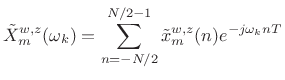
(8.6)
where , and
, and  is the sampling rate in
Hz. As in any FFT, we call
is the sampling rate in
Hz. As in any FFT, we call  the bin number.
- If needed, time normalization may be removed using a
linear phase term to yield the sampled STFT:
(8.7)
The (continuous-frequency) STFT may be approached arbitrarily closely by using more zero padding and/or other interpolation methods.Note that there is no irreversible time-aliasing when the STFT frequency axis
 is sampled to the points
  , provided
the FFT size
is greater than or equal to the window length
.
, provided
the FFT size
is greater than or equal to the window length
.
Two Dual Interpretations of the STFT
The STFT
![]() can be viewed as a function of either
frame-time
can be viewed as a function of either
frame-time ![]() or bin-frequency
or bin-frequency ![]() . We will develop both points of
view in this book.
. We will develop both points of
view in this book.
At each frame time ![]() , the STFT can be regarded as producing a
Fourier transform centered around that time. As
, the STFT can be regarded as producing a
Fourier transform centered around that time. As ![]() advances, a sequence of spectral transforms is obtained. This is
depicted graphically in Fig.9.1, and it forms the basis of the
overlap-add method for Fourier analysis, modification, and
resynthesis [9]. It is also the basis for
transform coders [16,284].
advances, a sequence of spectral transforms is obtained. This is
depicted graphically in Fig.9.1, and it forms the basis of the
overlap-add method for Fourier analysis, modification, and
resynthesis [9]. It is also the basis for
transform coders [16,284].
In an exact Fourier duality, each bin
![]() of the STFT can
be regarded as a sample of the complex signal at the output of a
lowpass filter whose input is
of the STFT can
be regarded as a sample of the complex signal at the output of a
lowpass filter whose input is
![]() . As discussed
in §9.1.2, this signal is obtained from
. As discussed
in §9.1.2, this signal is obtained from
![]() by
frequency-shifting it so that frequency
by
frequency-shifting it so that frequency ![]() is translated
down to 0
Hz. For each value of
is translated
down to 0
Hz. For each value of ![]() , the time-domain signal
, the time-domain signal
![]() , for
, for
![]() , is the output of
the
, is the output of
the ![]() th ``filter bank channel,'' for
th ``filter bank channel,'' for
![]() . In this
``filter bank'' interpretation, the hop size
. In this
``filter bank'' interpretation, the hop size ![]() can be interpreted as
the downsampling factor applied to each bin-filter output, and
the analysis window
can be interpreted as
the downsampling factor applied to each bin-filter output, and
the analysis window
![]() is seen as the impulse
response of the anti-aliasing filter used prior to downsampling. The
window transform
is seen as the impulse
response of the anti-aliasing filter used prior to downsampling. The
window transform ![]() is also the frequency response of each
channel filter (translated to dc). This point of view is depicted
graphically in Fig.9.2 and elaborated further in Chapter 9.
is also the frequency response of each
channel filter (translated to dc). This point of view is depicted
graphically in Fig.9.2 and elaborated further in Chapter 9.
The STFT as a Time-Frequency Distribution
The Short Time Fourier Transform (STFT)
![]() is a function
of both time (frame number
is a function
of both time (frame number ![]() ) and frequency (
) and frequency (
![]() ).
It is therefore an example of a time-frequency distribution.
Others include
).
It is therefore an example of a time-frequency distribution.
Others include
![\includegraphics[width=0.8\twidth]{eps/timefreq}](http://www.dsprelated.com/josimages_new/sasp2/img1287.png) |
STFT in Matlab
The following matlab segment illustrates the above processing steps:
Xtwz = zeros(N,nframes); % pre-allocate STFT output array
M = length(w);           % M = window length, N = FFT length
zp = zeros(N-M,1);       % zero padding (to be inserted)
xoff = 0;                % current offset in input signal x
Mo2 = (M-1)/2;           % Assume M odd for simplicity here
for m=1:nframes
  xt = x(xoff+1:xoff+M); % extract frame of input data
  xtw = w .* xt;         % apply window to current frame
  xtwz = [xtw(Mo2+1:M); zp; xtw(1:Mo2)]; % windowed, zero padded
  Xtwz(:,m) = fft(xtwz); % STFT for frame m
  xoff = xoff + R;       % advance in-pointer by hop-size R
end
Notes
- The window w is implemented in zero-centered
(``zero-phase'') form (see, e.g., §2.5.4 for discussion).
- The signal x should have at least Mo2 leading
zeros for this (simplified) implementation.
- See §F.3 for a more detailed implementation.
Next Section:
Classic Spectrograms
Previous Section:
The Panning Problem


