Sinusoidal Amplitude and Phase Estimation
The form of the optimal estimator (5.39) immediately suggests
the following generalization for the case of unknown amplitude and phase:
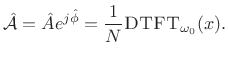
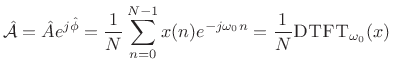 |
(6.41) |
That is,

is given by the
complex coefficient of
projection [
264] of

onto the complex
sinusoid

at the known frequency

. This can be shown by generalizing the
previous derivation, but here we will derive it using the more
enlightened
orthogonality principle [
114].
The orthogonality principle for linear least squares estimation states
that the projection error must be orthogonal to the model.
That is, if  is our optimal signal model (viewed now as an
 -vector in
  ), then we must have [264]
Thus, the complex coefficient of projection of
onto
 is given by
 |
(6.42) |
The optimality of
in the least squares sense follows from the
least-squares optimality of
orthogonal projection
[
114,
121,
252]. From a geometrical point of view,
referring to Fig.
5.16, we say that the minimum distance from a
vector

to some lower-dimensional subspace

, where

(here

for one
complex sinusoid) may be found by ``dropping
a
perpendicular'' from
to the subspace. The point
at the
foot of the
perpendicular is the point within the subspace closest to
in Euclidean distance.
Next Section: Sinusoidal Frequency EstimationPrevious Section: Sinusoidal Amplitude Estimation


