


Time-Frequency Displays
The preceding chapters have been concerned with the spectrum analysis of sinusoids and noise at a particular point in time (or a single spectrum for all time). This chapter introduces the Short-Time Fourier Transform (STFT)--a time-ordered sequence of spectral estimates, each using a finite-length analysis window. The STFT is used to compute the classic spectrogram, used extensively for speech and audio signals in general [132,57,199,162,226,74,81]. Finally, we point to methods for making spectrograms correspond better to audio perception, so that what you see is what you hear, to a greater extent. In particular, a loudness spectrogram based on a psychoacoustic model of time-varying loudness perception is described.
The Short-Time Fourier Transform
The Short-Time Fourier Transform (STFT) (or short-term Fourier transform) is a powerful general-purpose tool for audio signal processing [7,9,8]. It defines a particularly useful class of time-frequency distributions [43] which specify complex amplitude versus time and frequency for any signal. We are primarily concerned here with tuning the STFT parameters for the following applications:
- Approximating the time-frequency analysis performed by the ear for purposes of spectral display.
- Measuring model parameters in a short-time spectrum.
Examples of the second case include estimating the decay-time-versus-frequency for vibrating strings [288] and body resonances [119], or measuring as precisely as possible the fundamental frequency of a periodic signal [106] based on tracking its many harmonics in the STFT [64].
An interesting example for which cases 1 and 2 normally coincide is pitch detection (case 1) and fundamental frequency estimation (case 2). Here, ``fundamental frequency'' is defined as the lowest frequency present in a series of harmonic overtones, while ``pitch'' is defined as the perceived fundamental frequency; perceived pitch can be measured, for example, by comparing to a harmonic reference tone such as a sawtooth waveform. (Thus, by definition, the pitch of a sawtooth waveform is its fundamental frequency.) When harmonics are stretched so that they become slightly inharmonic, pitch perception corresponds to a (possibly non-existent) compromise fundamental frequency, the harmonics of which ``best fit'' the most audible overtones in some sense. The topic of ``pitch detection'' in the signal processing literature is often really about fundamental frequency estimation [106], and this distinction is lost. This is not a problem for strictly periodic signals.
Mathematical Definition of the STFT
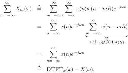
The usual mathematical definition of the STFT is
[9]
where

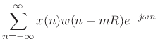
If the window ![]() has the
Constant OverLap-Add (COLA) property at hop-size
has the
Constant OverLap-Add (COLA) property at hop-size ![]() , i.e., if
, i.e., if
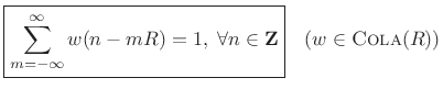
then the sum of the successive DTFTs over time equals the DTFT of the whole signal
We will say that windows satisfying
![]() (or some
constant) for all
(or some
constant) for all
![]() are said to be
are said to be
![]() . For example,
the length
. For example,
the length ![]() rectangular window is clearly
rectangular window is clearly
![]() (no overlap).
The Bartlett window and all windows in the generalized Hamming family
(Chapter 3) are
(no overlap).
The Bartlett window and all windows in the generalized Hamming family
(Chapter 3) are
![]() (50% overlap),
when the endpoints are handled correctly.8.1 A
(50% overlap),
when the endpoints are handled correctly.8.1 A
![]() example
is depicted in
Fig.8.9. Any window that is
example
is depicted in
Fig.8.9. Any window that is
![]() is also
is also
![]() ,
for
,
for
![]() , provided
, provided ![]() is an
integer.8.2 We will explore COLA windows
more completely in Chapter 8.
is an
integer.8.2 We will explore COLA windows
more completely in Chapter 8.
When using the short-time Fourier transform for signal processing, as taken up in Chapter 8, the COLA requirement is important for avoiding artifacts. For usage as a spectrum analyzer for measurement and display, the COLA requirement can often be relaxed, as doing so only means we are not weighting all information equally in our analysis. Nothing disastrous happens, for example, if we use 50% overlap with the Blackman window in a short-time spectrum analysis over time--the results look fine; however, in such a case, data falling near the edges of the window will have a slightly muted impact on the results relative to data falling near the window center, because the Blackman window is not COLA at 50% overlap.
Practical Computation of the STFT
While the definition of the STFT in (7.1) is useful for theoretical work, it is not really a specification of a practical STFT. In practice, the STFT is computed as a succession of FFTs of windowed data frames, where the window ``slides'' or ``hops'' forward through time. We now derive such an implementation of the STFT from its mathematical definition.
The STFT in (7.1) can be rewritten, adding ![]() to
to ![]() , as
, as
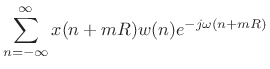
In this form, the data centered about time
Since indexing in the DFT is modulo
Summary of STFT Computation Using FFTs
- Read
 samples of the input signal
  into a local buffer of
length
into a local buffer of
length  which is initially zeroed
We call the
the  th frame of the input signal, and
 the
th time normalized input frame
(time-normalized by translating it to time zero). The frame length is
the
th time normalized input frame
(time-normalized by translating it to time zero). The frame length is
 , which we assume to be odd for reasons to be
discussed later. The time advance
, which we assume to be odd for reasons to be
discussed later. The time advance  (in samples) from one frame to
the next is called the
hop size
or
step size.
(in samples) from one frame to
the next is called the
hop size
or
step size.
- Multiply the data frame pointwise by a length
spectrum
analysis window
 to obtain the
th
windowed data frame (time normalized):
to obtain the
th
windowed data frame (time normalized):
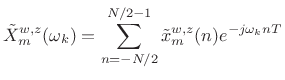
- Extend
 with zeros on both sides to obtain a
zero-padded frame:
with zeros on both sides to obtain a
zero-padded frame:
![$\displaystyle \tilde{x}_m^{w,z}(n) \isdef \left\{\begin{array}{ll} \tilde{x}_m^w(n), & \left\vert n\right\vert\leq M_h\isdef {\frac{M-1}{2}} \\ [5pt] 0, & M_h< n \leq {\frac{N}{2}}-1 \\ [5pt] 0, & -{\frac{N}{2}}\leq n < -M_h \\ \end{array} \right.$](http://www.dsprelated.com/josimages_new/sasp2/img1274.png)
(8.5)
where is chosen to be a power of two larger than
. The number
is chosen to be a power of two larger than
. The number
 is the
zero-padding factor.
As discussed in §2.5.3,
the zero-padding factor is the interpolation factor for the
spectrum, i.e., each FFT bin is replaced by
bins, interpolating
the spectrum using ideal bandlimited interpolation [264], where
the ``band'' in this case is the
-sample nonzero duration of
in the time domain.
is the
zero-padding factor.
As discussed in §2.5.3,
the zero-padding factor is the interpolation factor for the
spectrum, i.e., each FFT bin is replaced by
bins, interpolating
the spectrum using ideal bandlimited interpolation [264], where
the ``band'' in this case is the
-sample nonzero duration of
in the time domain.
- Take a length
FFT of
 to obtain the time-normalized,
frequency-sampled STFT at time
:
to obtain the time-normalized,
frequency-sampled STFT at time
:
(8.6)
where , and
, and  is the sampling rate in
Hz. As in any FFT, we call
is the sampling rate in
Hz. As in any FFT, we call  the bin number.
- If needed, time normalization may be removed using a
linear phase term to yield the sampled STFT:
(8.7)
The (continuous-frequency) STFT may be approached arbitrarily closely by using more zero padding and/or other interpolation methods.Note that there is no irreversible time-aliasing when the STFT frequency axis
 is sampled to the points
  , provided
the FFT size
is greater than or equal to the window length
.
, provided
the FFT size
is greater than or equal to the window length
.
Two Dual Interpretations of the STFT
The STFT
![]() can be viewed as a function of either
frame-time
can be viewed as a function of either
frame-time ![]() or bin-frequency
or bin-frequency ![]() . We will develop both points of
view in this book.
. We will develop both points of
view in this book.
At each frame time ![]() , the STFT can be regarded as producing a
Fourier transform centered around that time. As
, the STFT can be regarded as producing a
Fourier transform centered around that time. As ![]() advances, a sequence of spectral transforms is obtained. This is
depicted graphically in Fig.9.1, and it forms the basis of the
overlap-add method for Fourier analysis, modification, and
resynthesis [9]. It is also the basis for
transform coders [16,284].
advances, a sequence of spectral transforms is obtained. This is
depicted graphically in Fig.9.1, and it forms the basis of the
overlap-add method for Fourier analysis, modification, and
resynthesis [9]. It is also the basis for
transform coders [16,284].
In an exact Fourier duality, each bin
![]() of the STFT can
be regarded as a sample of the complex signal at the output of a
lowpass filter whose input is
of the STFT can
be regarded as a sample of the complex signal at the output of a
lowpass filter whose input is
![]() . As discussed
in §9.1.2, this signal is obtained from
. As discussed
in §9.1.2, this signal is obtained from
![]() by
frequency-shifting it so that frequency
by
frequency-shifting it so that frequency ![]() is translated
down to 0
Hz. For each value of
is translated
down to 0
Hz. For each value of ![]() , the time-domain signal
, the time-domain signal
![]() , for
, for
![]() , is the output of
the
, is the output of
the ![]() th ``filter bank channel,'' for
th ``filter bank channel,'' for
![]() . In this
``filter bank'' interpretation, the hop size
. In this
``filter bank'' interpretation, the hop size ![]() can be interpreted as
the downsampling factor applied to each bin-filter output, and
the analysis window
can be interpreted as
the downsampling factor applied to each bin-filter output, and
the analysis window
![]() is seen as the impulse
response of the anti-aliasing filter used prior to downsampling. The
window transform
is seen as the impulse
response of the anti-aliasing filter used prior to downsampling. The
window transform ![]() is also the frequency response of each
channel filter (translated to dc). This point of view is depicted
graphically in Fig.9.2 and elaborated further in Chapter 9.
is also the frequency response of each
channel filter (translated to dc). This point of view is depicted
graphically in Fig.9.2 and elaborated further in Chapter 9.
The STFT as a Time-Frequency Distribution
The Short Time Fourier Transform (STFT)
![]() is a function
of both time (frame number
is a function
of both time (frame number ![]() ) and frequency (
) and frequency (
![]() ).
It is therefore an example of a time-frequency distribution.
Others include
).
It is therefore an example of a time-frequency distribution.
Others include
![\includegraphics[width=0.8\twidth]{eps/timefreq}](http://www.dsprelated.com/josimages_new/sasp2/img1287.png) |
STFT in Matlab
The following matlab segment illustrates the above processing steps:
Xtwz = zeros(N,nframes); % pre-allocate STFT output array
M = length(w);           % M = window length, N = FFT length
zp = zeros(N-M,1);       % zero padding (to be inserted)
xoff = 0;                % current offset in input signal x
Mo2 = (M-1)/2;           % Assume M odd for simplicity here
for m=1:nframes
  xt = x(xoff+1:xoff+M); % extract frame of input data
  xtw = w .* xt;         % apply window to current frame
  xtwz = [xtw(Mo2+1:M); zp; xtw(1:Mo2)]; % windowed, zero padded
  Xtwz(:,m) = fft(xtwz); % STFT for frame m
  xoff = xoff + R;       % advance in-pointer by hop-size R
end
Notes
- The window w is implemented in zero-centered
(``zero-phase'') form (see, e.g., §2.5.4 for discussion).
- The signal x should have at least Mo2 leading
zeros for this (simplified) implementation.
- See §F.3 for a more detailed implementation.
Classic Spectrograms
The spectrogram is a basic tool in audio spectral analysis and other applications. It has been used extensively in speech analysis [56]. The spectrogram can be defined as an intensity plot (usually on a log scale, such as dB) of the Short-Time Fourier Transform (STFT) magnitude.8.4 As defined in the previous section, the STFT is simply a sequence of FFTs of windowed data segments, where the windows are allowed to overlap in time, typically by at least 50% [9]. Parameters of the spectrogram include the
- window length
,
- window type (Hamming, Kaiser, etc.),
- hop-size
, and
- FFT length
.
The spectrogram is an important representation of audio data because human hearing is based on a kind of real-time spectrogram encoded by the cochlea of the inner ear [199]. The spectrogram has been used extensively in the field of computer music as a guide during the development of sound synthesis algorithms. When working with an appropriate synthesis model, matching the spectrogram often corresponds to matching the sound extremely well. In fact, spectral modeling synthesis (SMS) is based on synthesizing the short-time spectrum directly by some means (see §10.4) [303].
Spectrogram of Speech
![\includegraphics[width=\twidth]{eps/speechspgm}](http://www.dsprelated.com/josimages_new/sasp2/img1289.png)
An example spectrogram for recorded speech data is shown in Fig.7.2. It was generated using the Matlab code displayed in Fig.7.3. The function spectrogram is listed in §F.3. The spectrogram is computed as a sequence of FFTs of windowed data segments. The spectrogram is plotted within spectrogram using imagesc.
[y,fs,bits] = wavread('SpeechSample.wav');
soundsc(y,fs); % Let's hear it
% for classic look:
colormap('gray'); map = colormap; imap = flipud(map);
M = round(0.02*fs);  % 20 ms window is typical
N = 2^nextpow2(4*M); % zero padding for interpolation
w = hamming(M);
spectrogram(y,N,fs,w,-M/8,1,60);
title('Speech Sample Spectrogram');
colormap(imap);
|
In this example, the Hamming window length was chosen to be 20 ms--a common choice in speech analysis. This is short enough so that any single 20 ms frame will typically contain data from only one phoneme, yet long enough that it will include at least two periods of the fundamental frequency during voiced speech, assuming the lowest voiced pitch to be around 100 Hz.
More generally, for speech and the singing voice (and any periodic tone), the STFT analysis parameters are chosen to trade off among the following conflicting criteria:
- The harmonics should be resolved.
- Pitch and formant variations should be closely followed.
Audio Spectrograms
Since classic spectrograms [132] typically show log-magnitude intensity (dB) versus time and frequency, and since sound-pressure level in dB is roughly proportional to perceived loudness, at least at high levels [179,276,305], we can say that a classic spectrogram provides a reasonably good psychoacoustic display for sound, provided the window length has been chosen to be comparable to the ``integration time'' of the ear.
However, there are several ways we can improve the classic spectrogram to obtain more psychoacoustically faithful displays of perceived loudness versus time and frequency:
- Loudness perception is closer to linearly related to
amplitude at low loudness levels.
- Since the STFT offers only one ``integration time'' (the window
length), it implements a uniform bandpass filter bank--i.e.,
spectral samples are uniformly spaced and correspond to equal
bandwidths. The window transform gives the shape of each effective
bandpass filter in the frequency domain. The choice of window length
determines the common time- and frequency-resolution at all
frequencies. Figure 9.14 shows a frequency-response overlay of
all 5 channel filters created by a length 5 DFT using a zero-phase
rectangular window.
In the ear, however, time resolution increases and frequency resolution decreases at higher frequencies. Thus, the ear implements a non-uniform filter bank, with wider bandwidths at higher frequencies. In the time domain, the integration time (effective ``window length'') becomes shorter at higher frequencies.
Auditory Filter Banks
Auditory filter banks are non-uniform bandpass filter banks designed to imitate the frequency resolution of human hearing [307,180,87,208,255]. Classical auditory filter banks include constant-Q filter banks such as the widely used third-octave filter bank. Digital constant-Q filter banks have also been developed for audio applications [29,30]. More recently, constant-Q filter banks for audio have been devised based on the wavelet transform, including the auditory wavelet filter bank [110]. Auditory filter banks have also been based more directly on psychoacoustic measurements, leading to approximations of the auditory filter frequency response in terms of a Gaussian function [205], a ``rounded exponential'' [207], and more recently the gammatone (or ``Patterson-Holdsworth'') filter bank [208,255]. The gamma-chirp filter bank further adds a level-dependent asymmetric correction to the basic gammatone channel frequency response, thus providing a more accurate approximation to the auditory frequency response [112,111].
The output power from an auditory filter bank at a particular time defines the so-called excitation pattern versus frequency at that time [87,179,305]. It may be considered analogous to the average power of the physical excitation applied to the hair cells of the inner ear by the vibrating basilar membrane in the cochlea.8.6 The shape of the excitation pattern can thus be thought of as approximating the envelope of the basilar membrane vibration.
The excitation pattern produced from an auditory filter bank, together with appropriate equalization (frequency-dependent gain) and nonlinear compression, can be used to define specific loudness as a function of time and frequency [306,305,177,182,88].
Because the channels of an auditory filter bank are distributed non-uniformly versus frequency, they can be regarded as a basis for a non-uniform sampling of the frequency axis. In this point of view, the auditory-filter frequency response becomes the (frequency-dependent) interpolation kernel used to extract a frequency sample at the filter's center frequency. See §7.3.3 below for further details.
Loudness Spectrogram
The purpose of a loudness spectrogram is to display some psychoacoustic model of loudness versus time and frequency. Instead of specifying FFT window length and type, one specifies conditions of presentation, such as physical amplitude level in dB SPL, angle of arrival at the ears, etc. By default, it can be assumed that the signal is presented to both ears equally, and the listening level can be normalized to a ``comfortable'' value such as 70 dB SPL.8.7
A time-varying model of loudness perception has been developed by Moore and Glasberg et al. [87,182,88]. A loudness spectrogram based on this work may consist of the following processing steps:
- Compute a multiresolution STFT (MRSTFT) which
approximates the frequency-dependent frequency and time resolution of
the ear. Several FFTs of different lengths may be combined in such a
way that time resolution is higher at high frequencies, and frequency
resolution is higher at low frequencies, like in the ear. In each
FFT, the frequency resolution must be greater than or equal to that of
the ear in the frequency band it covers. (Even ``much greater'' is ok,
since the resolution will be reduced down to what it should be by
smoothing in Step 2.)
- Form the excitation pattern from the MRSTFT by
resampling the FFTs of the previous step using interpolation kernels
shaped like auditory filters. The new spectral sampling intervals
should be proportional to the width of a critical band of
hearing at each frequency. The shape of each interpolation kernel
(auditory filter) should change with amplitude level as well as center
frequency [87]. This step effectively converts
the uniform filter bank of the FFT to an auditory filter
bank.8.8
- Compute the specific loudness from the excitation
pattern for each frame. This step implements a compressive
nonlinearity which depends on the frequency and level of the
excitation pattern
[182].
The specific loudness can be interpreted as loudness per ERB.
- If desired, the instantaneous loudness can be computed
as the the sum of the specific loudness over all frequency samples at
a fixed time. Similarly, short- and long-term time-varying loudness
estimates can be computed as lowpass-filterings of the instantaneous
loudness over time [88].
A Note on Hop Size
Before Step 2 above, the FFT hop size within the MRSTFT of Step 1 would typically be determined by the shortest window length used (and its type). However, after the non-uniform downsampling in Step 2, the effective window lengths (and shapes) have been modified. If the spectrum is not undersampled by this operation, the effective duration of the time-domain window at each frequency will always be shorter than that of the original FFT window. In principle, the shape of the effective time-domain window becomes the product of the original FFT window used in the MRSTFT times the ``auditory window,'' which is given by the inverse Fourier transform of the auditory filter frequency response (spectral interpolation kernel) translated to zero center-frequency. (This is only approximately true when the auditory filter frequency response spans multiple frequency ranges for which FFTs were performed at different resolutions.)
Since the time-domain window durations are shortened by the spectral
smoothing inherent in Step 2, the proper step size from frame to frame
is something less than that dictated by the MRSTFT windows. One
reliable method for determining the maximum allowable hop size for
each FFT in the MRSTFT is to study the inverse Fourier transform of
the widest (highest-frequency) auditory filter shape (translated to 0
Hz center-frequency) used as a smoothing kernel in that FFT. This new
window can be multiplied by the original window and overlapped and
added to itself, as in Eq.![]() (7.2), at various increasing
hop-sizes
(7.2), at various increasing
hop-sizes ![]() (starting with
(starting with ![]() which is always valid), until the
overlap-add begins to show ripple at the frame rate
which is always valid), until the
overlap-add begins to show ripple at the frame rate ![]() .
Alternatively, the bandwidth of the highest-frequency auditory filter
can be used to determine the appropriate hop size in the time domain,
as elaborated in Chapter 9 (especially §9.8.1).
.
Alternatively, the bandwidth of the highest-frequency auditory filter
can be used to determine the appropriate hop size in the time domain,
as elaborated in Chapter 9 (especially §9.8.1).
Loudness Spectrogram Examples
We now illustrate a particular Matlab implementation of a loudness spectrogram developed by teaching assistant Patty Huang, following [87,182,88] with slight modifications.8.9
Multiresolution STFT
Figure 7.4 shows a multiresolution STFT for the same
speech signal that was analyzed to produce Fig.7.2. The
bandlimits in Hz for the five combined FFTs were
![]() , where the last two (in
parentheses) were not used due to the signal sampling rate being only
, where the last two (in
parentheses) were not used due to the signal sampling rate being only
![]() kHz. The corresponding window lengths in milliseconds were
kHz. The corresponding window lengths in milliseconds were
![]() , where, again, the last two are not needed for
this example. Our hop size is chosen to be 1 ms, giving 75% overlap
in the highest-frequency channel, and more overlap in lower-frequency
channels. Thus, all frequency channels are oversampled along
the time dimension. Since many frequency channels from each FFT will
be combined via smoothing to form the ``excitation pattern'' (see next
section), temporal oversampling is necessary in all channels to avoid
uneven weighting of data in the time domain due to the hop size being
too large for the shortened effective time-domain windows.
, where, again, the last two are not needed for
this example. Our hop size is chosen to be 1 ms, giving 75% overlap
in the highest-frequency channel, and more overlap in lower-frequency
channels. Thus, all frequency channels are oversampled along
the time dimension. Since many frequency channels from each FFT will
be combined via smoothing to form the ``excitation pattern'' (see next
section), temporal oversampling is necessary in all channels to avoid
uneven weighting of data in the time domain due to the hop size being
too large for the shortened effective time-domain windows.
![\includegraphics[width=\twidth]{eps/lsg-mrstft}](http://www.dsprelated.com/josimages_new/sasp2/img1293.png) |
Excitation Pattern
Figure 7.5 shows the result of converting the MRSTFT to an excitation pattern [87,182,108]. As mentioned above, this essentially converts the MRSTFT into a better approximation of an auditory filter bank by non-uniformly resampling the frequency axis using auditory interpolation kernels.
Note that the harmonics are now clearly visible only up to approximately 20 ERBs, and only the first four or five harmonics are visible during voiced segments. During voiced segments, the formant structure is especially clearly visible at about 25 ERBs. Also note that ``pitch pulses'' are visible as very thin, alternating, dark and light vertical stripes above 25 ERBs or so; the dark lines occur just after glottal closure, when the voiced-speech period has a strong peak in the time domain.
![\includegraphics[width=\twidth]{eps/lsg-ep}](http://www.dsprelated.com/josimages_new/sasp2/img1294.png)
Nonuniform Spectral Resampling
Recall sinc interpolation of a discrete-time signal [270]:
And recall asinc interpolation of a sampled spectrum (§2.5.2):
![\begin{eqnarray*}
X(\omega) &=& \hbox{\sc DTFT}(\hbox{\sc ZeroPad}_{\infty}(\hbox{\sc IDFT}_N(X)))\\
&=& \sum_{k=0}^{N-1}X(\omega_k)\cdot \hbox{asinc}_N(\omega-\omega_k)\\ [5pt]
&=& (X\circledast \hbox{asinc}_N)_\omega,
\end{eqnarray*}](http://www.dsprelated.com/josimages_new/sasp2/img1296.png)
We see that resampling consists of an inner-product between the given samples with a continuous interpolation kernel that is sampled where needed to satisfy the needs of the inner product operation. In the time domain, our interpolation kernel is a scaled sinc function, while in the frequency domain, it is an asinc function. The interpolation kernel can of course be horizontally scaled to alter bandwidth [270], or more generally reshaped to introduce a more general windowing in the opposite domain:
- Width of interpolation kernel (main-lobe width)
 1/width-in-other-domain
- Shape of interpolation kernel
gain profile
(window) in other domain
Getting back to non-uniform resampling of audio spectra, we have that an auditory-filter frequency-response can be regarded as a frequency-dependent interpolation kernel for nonuniformly resampling the STFT frequency axis. In other words, an auditory filter bank may be implemented as a non-uniform resampling of the uniformly sampled frequency axis provided by an ordinary FFT, using the auditory filter shape as the interpolation kernel.
When the auditory filters vary systematically with frequency, there may be an equivalent non-uniform frequency-warping followed by a uniform sampling of the (warped) frequency axis. Thus, an alternative implementation of an auditory filter bank is to apply an FFT (implementing a uniform filter bank) to a signal having a properly prewarped spectrum, where the warping is designed to approximate whatever auditory frequency axis is desired. This approach is discussed further in Appendix E. (See also §2.5.2.)
Auditory Filter Shapes
The topic of auditory filter banks was introduced in §7.3.1 above. In this implementation, the auditory filters were synthesized from the Equivalent Rectangular Bandwidth (ERB) frequency scale, discussed in §E.5. The auditory filter-bank shapes are a function of level, so, ideally, the true physical amplitude level of the input signal at the ear(s) should be known. The auditory filter shape at 1 kHz in response to a sinusoidal excitation for a variety of amplitudes is shown in Fig.7.6.
![\includegraphics[width=4in]{eps/lsg-af}](http://www.dsprelated.com/josimages_new/sasp2/img1298.png)
Specific Loudness
Figure 7.7 shows the specific loudness computed from the excitation pattern of Fig.7.5. As mentioned above, it is a compressive nonlinearity that depends on level and also frequency.
![\includegraphics[width=\twidth]{eps/lsg-sl}](http://www.dsprelated.com/josimages_new/sasp2/img1299.png)
Spectrograms Compared
Figure 7.8 shows all four previous spectrogram figures in a two-by-two matrix for ease of cross-reference.
![\includegraphics[width=\twidth]{eps/lsg-fourcases}](http://www.dsprelated.com/josimages_new/sasp2/img1300.png) |
Instantaneous, Short-Term, and Long-Term Loudness
Finally, Fig.7.9 shows the instantaneous loudness, short-term loudness, and long-term loudness functions overlaid, for the same speech sample used in the previous plots. These are all single-valued functions of time which indicate the relative loudness of the signal on different time scales. See [88] for further discussion. While the lower plot looks reasonable, the upper plot (in sones) predicts only three audible time regions. Evidently, it corresponds to a very low listening level.8.10
The instantaneous loudness is simply the sum of the specific loudness over all frequencies. The short- and long-term loudnesses are derived by smoothing the instantaneous loudness with respect to time using various psychoacoustically motivated time constants [88]. The smoothing is nonlinear because the loudness tracks a rising amplitude very quickly, while decaying with a slower time constant.8.11 The loudness of a brief sound is taken to be the local maximum of the short-term loudness curve. The long-term loudness is related to loudness memory over time.
The upper plot gives loudness in sones, which is based on loudness perception experiments [276]; at 1 kHz and above, loudness perception is approximately logarithmic above 50 dB SPL or so, while below that, it tends toward being more linear. The lower plot is given in phons, which is simply sound pressure level (SPL) in dB at 1 kHz [276, p. 111]; at other frequencies, the amplitude in phons is defined by following an ``equal-loudness curve'' over to 1 kHz and reading off the level there in dB SPL. This means, e.g., that all pure tones have the same perceived loudness when they are at the same phon level, and the dB SPL at 1 kHz defines the loudness of such tones in phons.
![\includegraphics[width=4in]{eps/lsg-isl}](http://www.dsprelated.com/josimages_new/sasp2/img1301.png) |
Summary
In this chapter, we looked at a variety of time-frequency displays appropriate for audio signals. All were implemented in terms of the short-time Fourier transform (STFT). The classical spectrogram was reviewed, and its performance on a speech sample was illustrated. A loudness spectrogram based on a model of time-varying loudness perception [88] was discussed. In this model, the STFT (or a multiresolution STFT), is smoothed and non-uniformly resampled in frequency to approximate an auditory filter bank, whose power output is taken to be the excitation pattern. A compressive nonlinearity is then applied to produce the specific loudness, which we took as our loudness spectrogram. The specific loudness can be optionally smoothed with respect to time to form a short- or long-term loudness spectrogram. Summing over frequency yields the corresponding loudness functions versus time.
FFT-based non-uniform filter banks, providing more efficient loudness spectrograms, are discussed in §10.7.
Next Section:
Overlap-Add (OLA) STFT Processing
Previous Section:
Spectrum Analysis of Noise


