


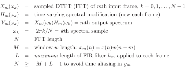
Time Varying OLA Modifications
In the preceding sections, we assumed that the spectral modification
![]() did not vary over time. We will now examine the implications of
time-varying spectral modifications. The derivation below
follows [9], except that we'll keep our previous
notation:
did not vary over time. We will now examine the implications of
time-varying spectral modifications. The derivation below
follows [9], except that we'll keep our previous
notation:
Using ![]() in our OLA formulation with a hop size
in our OLA formulation with a hop size ![]() results in
results in
![\begin{eqnarray*}
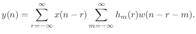
y(n) &=& \sum_{m=-\infty}^\infty y_m(n) \\
&=& \sum_{m=-\infty}^\infty \frac{1}{N}\sum_{k=0}^{N-1} X_m(\omega_k) H_m(\omega_k) e^{j\omega_kn} \\
&=& \sum_{m=-\infty}^\infty \frac{1}{N}\sum_{k=0}^{N-1}
\left[ \sum_{l=-\infty}^\infty x(l) w(l-m)e^{-j\omega_kl} \right]
H_m(\omega_k) e^{j\omega_kn} \\
&=& \sum_{l=-\infty}^\infty x(l) \sum_{m=-\infty}^\infty w(l-m)
\frac{1}{N}\sum_{k=0}^{N-1} H_m(\omega_k)
e^{j\omega_k(n-l)} \\
&=& \sum_{l=-\infty}^\infty x(l)
\sum_{m=-\infty}^\infty w(l-m) h_m(n-l) \\
\end{eqnarray*}](http://www.dsprelated.com/josimages_new/sasp2/img1499.png)
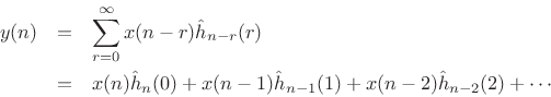
Define
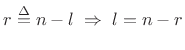 to get
 |
(9.42) |
Let's examine the term
 in more detail:
 describes the time variation of the
  tap.
tap.
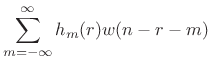
-
![$ \sum_{m=-\infty}^\infty h_m(r) w[(n-r)-m] = [h_{(\cdot)}(r) \ast w](n-r)$](http://www.dsprelated.com/josimages_new/sasp2/img1505.png) is a filtered version of the
tap
. It is
lowpass-filtered by w and delayed by
is a filtered version of the
tap
. It is
lowpass-filtered by w and delayed by  samples.
- Denote the
th time-varying, lowpass-filtered, delayed-by-
filter tap by
 . This can be interpreted
as the weighting in the output at time
of an impulse entering
the time-varying filter at time
. This can be interpreted
as the weighting in the output at time
of an impulse entering
the time-varying filter at time  .
.

This is a superposition sum for an arbitrary linear, time-varying filter
![]() .
.
Block Diagram Interpretation of Time-Varying STFT Modifications
Assuming ![]() is causal gives
is causal gives
This is depicted in Fig.8.17.
![\begin{psfrags}
% latex2html id marker 23334\psfrag{zm1}{\large $z^{-1}$\ }\psfrag{h(0,n)}{\large$ h_n(0) $}\psfrag{h(1,n)}{\large$ h_{n-1}(1) $}\psfrag{h(2,n)}{\large$ h_{n-L+1}(L-1) $}\psfrag{+}{\large$\Sigma$}\psfrag{w(n)}{\large$ w $}\psfrag{y(n)}{\large$ y(n) $}\begin{figure}[htbp]
\includegraphics[width=\twidth]{eps/olamods}
\caption{System diagram giving
an interpretation of the bandlimited time-varying filter coefficients
in the overlap-add STFT processor with a new filter each frame.}
\end{figure}
\end{psfrags}](http://www.dsprelated.com/josimages_new/sasp2/img1511.png)
The term ![]() can be interpreted as the FIR filter tap
can be interpreted as the FIR filter tap ![]() at time
at time
![]() . Note how each tap is lowpass filtered by the FFT window
. Note how each tap is lowpass filtered by the FFT window
![]() . The window thus enforces bandlimiting each filter tap to
the bandwidth of the window's main lobe. For an
. The window thus enforces bandlimiting each filter tap to
the bandwidth of the window's main lobe. For an ![]() -term length-
-term length-![]() Blackman-Harris window, for example, the main-lobe reaches zero at
frequency
Blackman-Harris window, for example, the main-lobe reaches zero at
frequency
![]() (see Table 5.2 in §5.5.2
for other examples). This bandlimiting places a limit on the bandwidth expansion
caused by time-variation of the filter coefficients, which in turn places a limit
on the maximum STFT hop-size that can be used without frequency-domain aliasing.
See Allen and Rabiner 1977
[9] for further details on the bandlimiting
property.
(see Table 5.2 in §5.5.2
for other examples). This bandlimiting places a limit on the bandwidth expansion
caused by time-variation of the filter coefficients, which in turn places a limit
on the maximum STFT hop-size that can be used without frequency-domain aliasing.
See Allen and Rabiner 1977
[9] for further details on the bandlimiting
property.
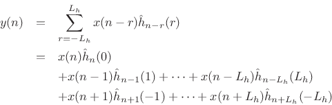
Length L FIR Frame Filters
To avoid time aliasing, we restrict the filter length to a maximum of
![]() samples. Since
samples. Since
![]() is an arbitrary multiplicative
weighting of the
is an arbitrary multiplicative
weighting of the ![]() th spectral frame, the frame filter need not be
causal. For odd
th spectral frame, the frame filter need not be
causal. For odd ![]() , the filter impulse response indices may run from
, the filter impulse response indices may run from
![]() to
to ![]() , where
, where
 |
(9.43) |
This gives
This is the general length ![]() time-varying FIR filter convolution sum for
time
time-varying FIR filter convolution sum for
time ![]() , when
, when ![]() is odd.
is odd.
Next Section:
Weighted Overlap Add
Previous Section:
Overlap-Save Method


