


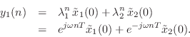
Choice of Output Signal and Initial Conditions
Recalling that
![]() , the output signal from any diagonal
state-space model is a linear combination of the modal signals. The
two immediate outputs
, the output signal from any diagonal
state-space model is a linear combination of the modal signals. The
two immediate outputs ![]() and
and ![]() in Fig.G.3 are given
in terms of the modal signals
in Fig.G.3 are given
in terms of the modal signals
![]() and
and
![]() as
as
![\begin{eqnarray*}
y_1(n) &=& [1, 0] {\underline{x}}(n) = [1, 0] \left[\begin{arr...
...\lambda_1^n {\tilde x}_1(0) - \eta \lambda_2^n\,{\tilde x}_2(0).
\end{eqnarray*}](http://www.dsprelated.com/josimages_new/filters/img2283.png)
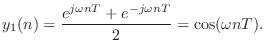
The output signal from the first state variable ![]() is
is
The initial condition
![]() corresponds to modal initial
state
corresponds to modal initial
state
![$\displaystyle \underline{{\tilde x}}(0) = E^{-1}\left[\begin{array}{c} 1 \\ [2p...
...nd{array}\right] = \left[\begin{array}{c} 1/2 \\ [2pt] 1/2 \end{array}\right].
$](http://www.dsprelated.com/josimages_new/filters/img2286.png)
Butterworth Lowpass Poles and Zeros
When the maximally flat optimality criterion is applied to the general
(analog) squared amplitude response
![]() , a surprisingly simple
result is obtained [64]:
, a surprisingly simple
result is obtained [64]:
where
The analytic continuation
(§D.2)
of
![]() to the whole
to the whole
![]() -plane may be obtained by substituting
-plane may be obtained by substituting
![]() to obtain
to obtain

with
A Butterworth lowpass filter additionally has ![]() zeros at
zeros at ![]() .
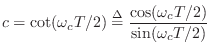
Under the bilinear transform
.
Under the bilinear transform
![]() , these all map to the
point
, these all map to the
point ![]() , which determines the numerator of the digital filter as
, which determines the numerator of the digital filter as
![]() .
.
Given the poles and zeros of the analog prototype, it is straightforward to convert to digital form by means of the bilinear transformation.
Example: Second-Order Butterworth Lowpass
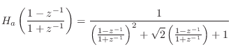
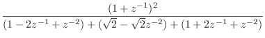
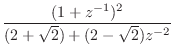
In the second-order case, we have, for the analog prototype,
To convert this to digital form, we apply the bilinear transform

 |
(I.4) | ||
 |
(I.5) | ||
 |
(I.6) | ||
 |
(I.7) |
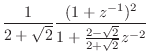
Note that the numerator is

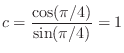
In the analog prototype,
the cut-off frequency is
![]() rad/sec, where,
from Eq.
rad/sec, where,
from Eq.![]() (I.1), the amplitude response
is
(I.1), the amplitude response
is
![]() . Since we mapped the cut-off frequency precisely
under the bilinear transform, we expect the digital filter to have
precisely this gain.
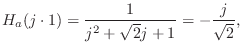
The digital frequency response at one-fourth the sampling rate is
. Since we mapped the cut-off frequency precisely
under the bilinear transform, we expect the digital filter to have
precisely this gain.
The digital frequency response at one-fourth the sampling rate is
and
Note from Eq.![]() (I.8) that the phase at cut-off is exactly -90 degrees
in the digital filter. This can be verified against the pole-zero
diagram in the
(I.8) that the phase at cut-off is exactly -90 degrees
in the digital filter. This can be verified against the pole-zero
diagram in the ![]() plane, which has two zeros at
plane, which has two zeros at ![]() , each
contributing +45 degrees, and two poles at
, each
contributing +45 degrees, and two poles at
![]() , each contributing -90
degrees. Thus, the calculated phase-response at the cut-off frequency
agrees with what we expect from the digital pole-zero diagram.
, each contributing -90
degrees. Thus, the calculated phase-response at the cut-off frequency
agrees with what we expect from the digital pole-zero diagram.
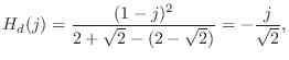
In the ![]() plane, it is not as easy to use the pole-zero diagram
to calculate the phase at
plane, it is not as easy to use the pole-zero diagram
to calculate the phase at
![]() , but using Eq.
, but using Eq.![]() (I.3), we
quickly obtain
(I.3), we
quickly obtain
A related example appears in §9.2.4.
Next Section:
Bilinear Transformation
Previous Section:
Finding the Eigenstructure of A


