


Complex Resonator
Normally when we need a resonator, we think immediately of the two-pole resonator. However, there is also a complex one-pole resonator having the transfer function
where
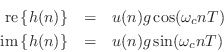
Since the impulse response is the inverse z transform of the
transfer function, we can write down the impulse response of the
complex one-pole resonator by recognizing Eq.![]() (B.6) as the
closed-form sum of an infinite geometric series, yielding
(B.6) as the
closed-form sum of an infinite geometric series, yielding
![$\displaystyle u(n) \isdef \left\{\begin{array}{ll}
1, & n\geq 0 \\ [5pt]
0, & n<0 \\
\end{array}\right.
$](http://www.dsprelated.com/josimages_new/filters/img1406.png)
These may be called phase-quadrature sinusoids, since their phases differ by 90 degrees. The phase quadrature relationship for two sinusoids means that they can be regarded as the real and imaginary parts of a complex sinusoid.
By allowing ![]() to be complex,
to be complex,
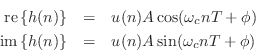
The frequency response of the complex one-pole resonator differs from
that of the two-pole real resonator in that the resonance
occurs only for one positive or negative frequency ![]() , but not
both. As a result, the resonance frequency
, but not
both. As a result, the resonance frequency ![]() is also the
frequency where the peak-gain occurs; this is only true in
general for the complex one-pole resonator. In particular, the peak
gain of a real two-pole filter does not occur exactly at resonance, except
when
is also the
frequency where the peak-gain occurs; this is only true in
general for the complex one-pole resonator. In particular, the peak
gain of a real two-pole filter does not occur exactly at resonance, except
when
![]() ,
, ![]() , or
, or ![]() . See
§B.6 for more on peak-gain versus resonance-gain (and how to
normalize them in practice).
. See
§B.6 for more on peak-gain versus resonance-gain (and how to
normalize them in practice).
Two-Pole Partial Fraction Expansion
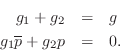
Note that every real two-pole resonator can be broken up into a sum of two complex one-pole resonators:
where
![\includegraphics[width=\twidth ]{eps/tppfe}](http://www.dsprelated.com/josimages_new/filters/img1419.png) |
To show Eq.![]() (B.7) is always true, let's solve in general for
(B.7) is always true, let's solve in general for ![]() and
and ![]() given
given ![]() and
and ![]() . Recombining the right-hand side
over a common denominator and equating numerators gives
. Recombining the right-hand side
over a common denominator and equating numerators gives
The solution is easily found to be
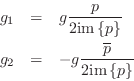
where we have assumed
im![]() , as necessary to have a
resonator in the first place.
, as necessary to have a
resonator in the first place.
Breaking up the two-pole real resonator into a parallel sum of two complex one-pole resonators is a simple example of a partial fraction expansion (PFE) (discussed more fully in §6.8).
Note that the inverse z transform of a sum of one-pole transfer
functions can be easily written down by inspection. In particular,
the impulse response of the PFE of the two-pole resonator (see
Eq.![]() (B.7)) is clearly
(B.7)) is clearly
Next Section:
The BiQuad Section
Previous Section:
Two-Zero


