


Finite Impulse Response Digital Filters
In §5.1 we defined the general difference equation for IIR filters, and a couple of second-order examples were diagrammed in Fig.5.1. In this section, we take a more detailed look at the special case of Finite Impulse Response (FIR) digital filters. In addition to introducing various terminology and practical considerations associated with FIR filters, we'll look at a preview of transfer-function analysis (Chapter 6) for this simple special case.
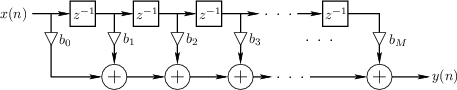 |
Figure 5.5 gives the signal flow graph for a general causal FIR filter Such a filter is also called a transversal filter, or a tapped delay line. The implementation shown is classified as a direct-form implementation.
FIR impulse response
The impulse response ![]() is obtained at the output when the
input signal is the impulse signal
is obtained at the output when the
input signal is the impulse signal
![]() (§5.6). If the
(§5.6). If the ![]() th tap is denoted
th tap is denoted ![]() , then it is
obvious from Fig.5.5 that the impulse response signal is
given by
, then it is
obvious from Fig.5.5 that the impulse response signal is
given by
![$\displaystyle h(n)\isdef \left\{\begin{array}{ll} 0, & n<0 \\ [5pt] b_n, & 0\leq n\leq M \\ [5pt] 0, & n> M \\ \end{array} \right. \protect$](http://www.dsprelated.com/josimages_new/filters/img596.png)
In other words, the impulse response simply consists of the tap coefficients, prepended and appended by zeros.
Convolution Representation of FIR Filters
Notice that the output of the ![]() th delay element in Fig.5.5 is
th delay element in Fig.5.5 is
![]() ,
,
![]() , where
, where ![]() is the input signal
amplitude at time
is the input signal
amplitude at time ![]() . The output signal
. The output signal ![]() is therefore
is therefore
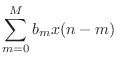
where we have used the convolution operator ``
The ``Finite'' in FIR
From Eq.![]() (5.7), we can see that the impulse response becomes zero
after time
(5.7), we can see that the impulse response becomes zero
after time ![]() . Therefore, a tapped delay line (Fig.5.5) can
only implement finite-duration impulse responses in the sense
that the non-zero portion of the impulse response must be finite.
This is what is meant by the term finite impulse response
(FIR). We may say that the impulse response has finite support
[52].
. Therefore, a tapped delay line (Fig.5.5) can
only implement finite-duration impulse responses in the sense
that the non-zero portion of the impulse response must be finite.
This is what is meant by the term finite impulse response
(FIR). We may say that the impulse response has finite support
[52].
Causal FIR Filters
From Eq.![]() (5.6), we see also that the impulse response
(5.6), we see also that the impulse response ![]() is
always zero for
is
always zero for ![]() . Recall from §5.3 that any LTI
filter having a zero impulse response prior to time 0 is said to be
causal. Thus, a tapped delay line such as that depicted in
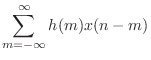
Fig.5.5 can only implement causal FIR filters. In software,
on the other hand, we may easily implement non-causal FIR filters as
well, based simply on the definition of convolution.
. Recall from §5.3 that any LTI
filter having a zero impulse response prior to time 0 is said to be
causal. Thus, a tapped delay line such as that depicted in
Fig.5.5 can only implement causal FIR filters. In software,
on the other hand, we may easily implement non-causal FIR filters as
well, based simply on the definition of convolution.
FIR Transfer Function
The transfer function of an FIR filter is given by the z transform of
its impulse response. This is true for any LTI filter, as discussed
in Chapter 6. For FIR filters in particular, we have, from
Eq.![]() (5.6),
(5.6),
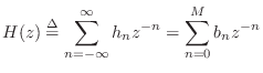
Thus, the transfer function of every length
FIR Order
The order of a filter is defined as the order of its transfer
function, as discussed in Chapter 6. For FIR filters, this is just
the order of the transfer-function polynomial. Thus, from
Equation (5.8), the order of the general, causal, length ![]() FIR
filter is
FIR
filter is ![]() (provided
(provided ![]() ).
).
Note from Fig.5.5 that the order ![]() is also the total number
of delay elements in the filter. This is typical of practical
digital filter implementations. When the number of delay elements in
the implementation (Fig.5.5) is equal to the filter order, the
filter implementation is said to be canonical with respect to
delay. It is not possible to implement a given transfer function in
fewer delays than the transfer function order, but it is possible (and
sometimes even desirable) to have extra delays.
is also the total number
of delay elements in the filter. This is typical of practical
digital filter implementations. When the number of delay elements in
the implementation (Fig.5.5) is equal to the filter order, the
filter implementation is said to be canonical with respect to
delay. It is not possible to implement a given transfer function in
fewer delays than the transfer function order, but it is possible (and
sometimes even desirable) to have extra delays.
FIR Software Implementations
In matlab, an efficient FIR filter is implemented by calling
outputsignal = filter(B,1,inputsignal);
where
Figure 5.6 lists a second-order FIR filter implementation in the C programming language.
typedef double *pp; // pointer to array of length NTICK typedef double word; // signal and coefficient data type typedef struct _fir3Vars { pp outputAout; pp inputAinp; word b0; word b1; word b2; word s1; word s2; } fir3Vars; void fir3(fir3Vars *a) { int i; word input; for (i=0; i<NTICK; i++) { input = a->inputAinp[i]; a->outputAout[i] = a->b0 * input + a->b1 * a->s1 + a->b2 * a->s2; a->s2 = a->s1; a->s1 = input; } } |
Next Section:
Transient Response, Steady State, and Decay
Previous Section:
Convolution Representation


