


Matlab Analysis of the Simplest Lowpass Filter
The example filter implementation listed in Fig.1.3 was written in the C programming language so that all computational details would be fully specified. However, C is a relatively low-level language for signal-processing software. Higher level languages such as matlab make it possible to write powerful programs much faster and more reliably. Even in embedded applications, for which assembly language is typically required, it is usually best to develop and debug the system in matlab beforehand.
The Matlab (R) product by The Mathworks, Inc., is far and away the richest implementation of the matlab language. However, it is very expensive for non-students, so you may at some point want to consider the free, open-source alternative called Octave. All examples in this chapter will work in either Matlab or Octave,3.1except that some plot-related commands may need to be modified. The term matlab (not capitalized) will refer henceforth to either Matlab or Octave, or any other compatible implementation of the matlab language.3.2
This chapter provides four matlab programming examples to complement the mathematical analysis of §1.3:
- 2.1:
- Filter implementation
- 2.2:
- Simulated sine-wave analysis
- 2.3:
- Simulated complex sine-wave analysis
- 2.4:
- Practical frequency-response analysis
Note: The reader is expected to know (at least some) matlab before proceeding. See, for example, the Matlab Getting Started documentation, or just forge ahead and use the examples below to start learning matlab. (It is very readable, as computer languages go.) To skip over the matlab examples for now, proceed to Chapter 3.
Matlab Filter Implementation
In this section, we will implement (in matlab) the simplest lowpass filter
- Fig.1.3 listed simplp for filtering one block of data, and
- Fig.1.4 listed a main program for testing simplp.
y = filter (B, A, x)
where
- x is the input signal (a vector of any length),
- y is the output signal (returned equal in length to x),
- A is a vector of filter feedback coefficients, and
- B is a vector of filter feedforward coefficients.
where
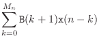
Note that Eq.![]() (2.1) could be written directly in matlab using two
for loops (as shown in Fig.3.2). However, this
would execute much slower because the matlab language is
interpreted, while built-in functions such as filter
are pre-compiled C modules. As a general rule, matlab programs should
avoid iterating over individual samples whenever possible. Instead,
whole signal vectors should be processed using expressions involving
vectors and matrices. In other words, algorithms should be
``vectorized'' as much as possible.
Accordingly, to get the most out of matlab, it is necessary to know
some linear algebra [58].
(2.1) could be written directly in matlab using two
for loops (as shown in Fig.3.2). However, this
would execute much slower because the matlab language is
interpreted, while built-in functions such as filter
are pre-compiled C modules. As a general rule, matlab programs should
avoid iterating over individual samples whenever possible. Instead,
whole signal vectors should be processed using expressions involving
vectors and matrices. In other words, algorithms should be
``vectorized'' as much as possible.
Accordingly, to get the most out of matlab, it is necessary to know
some linear algebra [58].
The simplest lowpass filter of Eq.![]() (1.1) is nonrecursive
(no feedback), so the feedback coefficient vector A is set to
1.3.5 Recursive filters will be
introduced later in §5.1. The minus sign in
Eq.
(1.1) is nonrecursive
(no feedback), so the feedback coefficient vector A is set to
1.3.5 Recursive filters will be
introduced later in §5.1. The minus sign in
Eq.![]() (2.1) will make sense after we study
filter transfer functions in Chapter 6.
(2.1) will make sense after we study
filter transfer functions in Chapter 6.
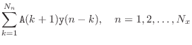
The feedforward coefficients needed for the simplest lowpass filter are
With these settings, the filter function implements
% simplpm1.m - matlab main program implementing
%              the simplest lowpass filter:
%
%                    y(n) = x(n)+x(n-1)}

N=10;       % length of test input signal
x = 1:N;    % test input signal (integer ramp)
B = [1,1];  % transfer function numerator
A = 1;      % transfer function denominator

y = filter(B,A,x);

for i=1:N
  disp(sprintf('x(%d)=%f\ty(%d)=%f',i,x(i),i,y(i)));
end

% Output:
%   octave:1> simplpm1
%   x(1)=1.000000       y(1)=1.000000
%   x(2)=2.000000       y(2)=3.000000
%   x(3)=3.000000       y(3)=5.000000
%   x(4)=4.000000       y(4)=7.000000
%   x(5)=5.000000       y(5)=9.000000
%   x(6)=6.000000       y(6)=11.000000
%   x(7)=7.000000       y(7)=13.000000
%   x(8)=8.000000       y(8)=15.000000
%   x(9)=9.000000       y(9)=17.000000
%   x(10)=10.000000     y(10)=19.000000
|
A main test program analogous to Fig.1.4 is shown in Fig.2.1. Note that the input signal is processed in one big block, rather than being broken up into two blocks as in Fig.1.4. If we want to process a large sound file block by block, we need some way to initialize the state of the filter for each block using the final state of the filter from the preceding block. The filter function accommodates this usage with an additional optional input and output argument:
[y, Sf] = filter (B, A, x, Si)
Si denotes the filter initial state, and
Sf denotes its final state. A main program illustrating
block-oriented processing is given in Fig.2.2.
% simplpm2.m - block-oriented version of simplpm1.m

N=10;       % length of test input signal
NB=N/2;     % block length
x = 1:N;    % test input signal
B = [1,1];  % feedforward coefficients
A = 1;      % feedback coefficients (no-feedback case)

[y1, Sf] = filter(B,A,x(1:NB));      % process block 1
      y2 = filter(B,A,x(NB+1:N),Sf); % process block 2

for i=1:NB   % print input and output for block 1
  disp(sprintf('x(%d)=%f\ty(%d)=%f',i,x(i),i,y1(i)));
end

for i=NB+1:N % print input and output for block 2
  disp(sprintf('x(%d)=%f\ty(%d)=%f',i,x(i),i,y2(i-NB)));
end
|
Simulated Sine-Wave Analysis in Matlab
In this section, we will find the frequency response of the simplest lowpass filter
% swanalmain.m - matlab program for simulated sine-wave % analysis on the simplest lowpass filter: % % y(n) = x(n)+x(n-1)} B = [1,1]; % filter feedforward coefficients A = 1; % filter feedback coefficients (none) N=10; % number of sinusoidal test frequencies fs = 1; % sampling rate in Hz (arbitrary) fmax = fs/2; % highest frequency to look at df = fmax/(N-1);% spacing between frequencies f = 0:df:fmax; % sampled frequency axis dt = 1/fs; % sampling interval in seconds tmax = 10; % number of seconds to run each sine test t = 0:dt:tmax; % sampled time axis ampin = 1; % test input signal amplitude phasein = 0; % test input signal phase [gains,phases] = swanal(t,f/fs,B,A); % sine-wave analysis swanalmainplot; % final plots and comparison to theory |
function [gains,phases] = swanal(t,f,B,A) % SWANAL - Perform sine-wave analysis on filter B(z)/A(z) ampin = 1; % input signal amplitude phasein = 0; % input signal phase N = length(f); % number of test frequencies gains = zeros(1,N); % pre-allocate amp-response array phases = zeros(1,N); % pre-allocate phase-response array if length(A)==1 ntransient=length(B)-1; % no. samples to steady state else error('Need to set transient response duration here'); end for k=1:length(f) % loop over analysis frequencies s = ampin*cos(2*pi*f(k)*t+phasein); % test sinusoid y = filter(B,A,s); % run it through the filter yss = y(ntransient+1:length(y)); % chop off transient % measure output amplitude as max (SHOULD INTERPOLATE): [ampout,peakloc] = max(abs(yss)); % ampl. peak & index gains(k) = ampout/ampin; % amplitude response if ampout < eps % eps returns "machine epsilon" phaseout=0; % phase is arbitrary at zero gain else sphase = 2*pi*f(k)*(peakloc+ntransient-1); % compute phase by inverting sinusoid (BAD METHOD): phaseout = acos(yss(peakloc)/ampout) - sphase; phaseout = mod2pi(phaseout); % reduce to [-pi,pi) end phases(k) = phaseout-phasein; swanalplot; % signal plotting script end |
In the swanal function (Fig.2.4), test sinusoids are generated by the line
s = ampin * cos(2*pi*f(k)*t + phasein);
where amplitude, frequency (Hz), and phase (radians) of the sinusoid are given be
ampin, f(k), and phasein, respectively. As discussed
in §1.3, assuming linearity and time-invariance (LTI) allows
us to set
        ampin = 1;      % input signal amplitude
        phasein = 0;    % input signal phase
without loss of generality. (Note that we must also assume the filter
is LTI for sine-wave analysis to be a general method for
characterizing the filter's response.) The test sinusoid is passed
through the digital filter by the line
y = filter(B,A,s); % run s through the filter
producing the output signal in vector y. For this example
(the simplest lowpass filter), the filter coefficients are simply
        B = [1,1]; % filter feedforward coefficients
        A = 1;     % filter feedback coefficients (none)
The coefficient A(1) is technically a coefficient on the
output signal itself, and it should always be normalized to 1.
(B and A can be multiplied by the same nonzero constant to
carry out this normalization when necessary.)
Figure 2.5 shows one of the intermediate plots produced by the
sine-wave analysis routine in Fig.2.4. This figure corresponds
to Fig.1.6 in §1.3 (see page ![]() ). In
Fig.2.5a, we see samples of the input test sinusoid overlaid
with the continuous sinusoid represented by those
samples. Figure 2.5b shows only the samples of the filter output
signal: While we know the output signal becomes a sampled sinusoid
after the one-sample transient response, we do not know its amplitude
or phase until we measure it; the underlying continuous signal
represented by the samples is therefore not plotted. (If we really
wanted to see this, we could use software for bandlimited
interpolation [91], such as Matlab's
interp function.) A plot such as Fig.2.5 is produced
for each test frequency, and the relative amplitude and phase are
measured between the input and output to form one sample of the
measured frequency response, as discussed in
§1.3.
). In
Fig.2.5a, we see samples of the input test sinusoid overlaid
with the continuous sinusoid represented by those
samples. Figure 2.5b shows only the samples of the filter output
signal: While we know the output signal becomes a sampled sinusoid
after the one-sample transient response, we do not know its amplitude
or phase until we measure it; the underlying continuous signal
represented by the samples is therefore not plotted. (If we really
wanted to see this, we could use software for bandlimited
interpolation [91], such as Matlab's
interp function.) A plot such as Fig.2.5 is produced
for each test frequency, and the relative amplitude and phase are
measured between the input and output to form one sample of the
measured frequency response, as discussed in
§1.3.
![\includegraphics[width=\twidth ]{eps/swanalsix}](http://www.dsprelated.com/josimages_new/filters/img258.png) |
Next, the one-sample start-up transient is removed from the filter
output signal y to form the ``cropped'' signal yss
(``![]() steady state''). The final task is to measure the amplitude
and phase of the yss. Output amplitude estimation is done in
swanal by the line
steady state''). The final task is to measure the amplitude
and phase of the yss. Output amplitude estimation is done in
swanal by the line
[ampout,peakloc] = max(abs(yss));
Note that the peak amplitude found in this way is approximate,
since the true peak of the output sinusoid generally occurs
between samples. We will find the output amplitude much
more accurately in the next two sections. We store the index of the
amplitude peak in peakloc so it can be used to estimate phase
in the next step. Given the output amplitude ampout, the
amplitude response of the filter at frequency f(k) is
given by
gains(k) = ampout/ampin;
The last step of swanal in Fig.2.4 is to estimate the
phase of the cropped filter output signal yss. Since we will
have better ways to accomplish this later, we use a simplistic method
here based on inverting the sinusoid analytically:
        phaseout = acos(yss(peakloc)/ampout) ...
                     - 2*pi*f(k)*(peakloc+ntransient-1);
        phaseout = mod2pi(phaseout); % reduce to [-pi,pi)
Again, this is only an approximation since peakloc is only
accurate to the nearest sample. The mod2pi utility reduces
its scalar argument to the range
function [y] = mod2pi(x) % MOD2PI - Reduce x to the range [-pi,pi) y=x; twopi = 2*pi; while y >= pi, y = y - twopi; end while y < -pi, y = y + twopi; end |
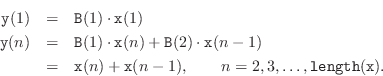
In summary, the sine-wave analysis measures experimentally the gain and phase-shift of the digital filter at selected frequencies, thus measuring the frequency response of the filter at those frequencies. It is interesting to compare these experimental results with the closed-form expressions for the frequency response derived in §1.3.2. From Equations (1.6-1.7) we have
where ![]() denotes the amplitude response (filter gain versus
frequency),
denotes the amplitude response (filter gain versus
frequency), ![]() denotes the phase response (filter
phase-shift versus frequency),
denotes the phase response (filter
phase-shift versus frequency), ![]() is frequency in Hz, and
is frequency in Hz, and ![]() denotes the sampling rate. Both the amplitude response and phase
response are real-valued functions of (real) frequency, while
the frequency response is the complex function of
frequency given by
denotes the sampling rate. Both the amplitude response and phase
response are real-valued functions of (real) frequency, while
the frequency response is the complex function of
frequency given by
![]() .
.
Figure 2.7 shows overlays of the measured and theoretical results. While there is good general agreement, there are noticeable errors in the measured amplitude and phase-response curves. Also, the phase-response error tends to be large when there is an amplitude response error, since the phase calculation used depends on knowledge of the amplitude response.
![\includegraphics[width=\twidth ]{eps/swanalmain}](http://www.dsprelated.com/josimages_new/filters/img267.png)
It is important to understand the source(s) of deviation between the measured and theoretical values. Our simulated sine-wave analysis deviates from an ideal sine-wave analysis in the following ways (listed in ascending order of importance):
- The test sinusoids are sampled instead of being
continuous in time: It turns out this is a problem only for frequencies
at half the sampling rate and above. Below half the sampling rate,
sampled sinusoids contain exactly the same information as continuous
sinusoids, and there is no penalty whatsoever associated with
discrete-time sampling itself.
- The test sinusoid samples are rounded to a
finite precision: Digitally sampled sinusoids do suffer from a
certain amount of round-off error, but Matlab and Octave use
double-precision floating-point numbers by default (64 bits). As a
result, our samples are far more precise than could be measured
acoustically in the physical world. This is not a visible source of
error in Fig.2.7.
- Our test sinusoids are finite duration, while the ideal
sinusoid is infinitely long: This can be a real practical limitation.
However, we worked around it completely by removing the start-up
transient. For the simplest lowpass filter, the start-up transient is
only one sample long. More generally, for digital filters expressible
as a weighted sum of
 successive samples (any nonrecursive
LTI digital filter), the start-up transient is
successive samples (any nonrecursive
LTI digital filter), the start-up transient is  samples long.
When we consider recursive digital filters, which employ output
feedback, we will no longer be able to remove the start-up transient
exactly, because it generally decays
exponentially instead of being finite in length. However, even
in that case, as long as the recursive filter is stable, we can define
the start-up transient as some number of time-constants of exponential
decay, thereby making the approximation error as small as we wish,
such as less than the round-off error.
samples long.
When we consider recursive digital filters, which employ output
feedback, we will no longer be able to remove the start-up transient
exactly, because it generally decays
exponentially instead of being finite in length. However, even
in that case, as long as the recursive filter is stable, we can define
the start-up transient as some number of time-constants of exponential
decay, thereby making the approximation error as small as we wish,
such as less than the round-off error.
- We measured the output amplitude and phase at a signal
peak measured only to the nearest sample: This is the major
source of error in our simulation. The program of Fig.2.3
measures the filter output amplitude very crudely as the maximum
magnitude. In general, even for this simple filter, the maximum
output signal amplitude occurs
between samples. To measure this, we would need to use what is
called bandlimited interpolation [91]. It
is possible and practical to make the error arbitrarily small by
increasing the sampling rate by some factor and finishing with
quadratic interpolation of the three samples about the peak magnitude.
Similar remarks apply to the measured output phase.
The need for interpolation is lessened greatly if the sampling rate is chosen to be unrelated to the test frequencies (ideally so that the number of samples in each sinusoidal period is an irrational number). Figure 2.8 shows the measured and theoretical results obtained by changing the highest test frequency fmax from
 to
to
 , and the number of samples in each test sinusoid
tmax from
, and the number of samples in each test sinusoid
tmax from  to
to  . For these parameters, at least one
sample falls very close to a true peak of the output sinusoid at each
test frequency.
. For these parameters, at least one
sample falls very close to a true peak of the output sinusoid at each
test frequency.
It should also be pointed out that one never estimates signal phase in practice by inverting the closed-form functional form assumed for the signal. Instead, we should estimate the delay of each output sinusoid relative to the corresponding input sinusoid. This leads to the general topic of time delay estimation [12]. Under the assumption that the round-off error can be modeled as ``white noise'' (typically this is an accurate assumption), the optimal time-delay estimator is obtained by finding the (interpolated) peak of the cross-correlation between the input and output signals. For further details on cross-correlation, a topic in statistical signal processing, see, e.g., [77,87].
Using the theory presented in later chapters, we will be able to compute very precisely the frequency response of any LTI digital filter without having to resort to bandlimited interpolation (for measuring amplitude response) or time-delay estimation (for measuring phase).
![\includegraphics[width=\twidth ]{eps/swanalrmain}](http://www.dsprelated.com/josimages_new/filters/img272.png)
Complex Sine-Wave Analysis
To illustrate the use of complex numbers in matlab, we repeat the previous sine-wave analysis of the simplest lowpass filter using complex sinusoids instead of real sinusoids.
Only the sine-wave analysis function needs to be rewritten, and it appears in Fig.2.10. The initial change is to replace the line
s = ampin * cos(2*pi*f(k)*t + phasein); % real sinusoidwith the line
s = ampin * e .^ (j*2*pi*f(k)*t + phasein); % complexAnother change in Fig.2.10 is that the plotsignals option is omitted, since a complex signal plot requires two real plots. This option is straightforward to restore if desired.
In the complex-sinusoid case, we find that measuring the amplitude and phase of the output signal is greatly facilitated. While we could use the previous method on either the real part or imaginary part of the complex output sinusoid, it is much better to measure its instananeous amplitude and instananeous phase by means of the formulas
Furthermore, since we should obtain the same answer for each sample, we can average the results to minimize noise due to round-off error:
  ampout = mean(abs(yss)); % avg instantaneous amplitude
  gains(k) = ampout/ampin; % amplitude response sample
  sss = s(ntransient+1:length(y)); % chop input like output
  phases(k) = mean(mod2pi(angle(yss.*conj(sss))));
The expression angle(yss.*conj(sss)) in the last line above produces a vector of estimated filter phases which are the same for each sample (to within accumulated round-off errors), because the term
The final measured frequency response is plotted in Fig.2.9.
The test conditions were as in Fig.2.7, i.e., the highest
test frequency was fmax = ![]() , and the number of samples
in each test sinusoid was tmax
, and the number of samples
in each test sinusoid was tmax ![]() . Unlike the real
sine-wave analysis results in Fig.2.7, there is no visible
error associated with complex sine-wave analysis. Because
instantaneous amplitude and phase are available from every sample of a
complex sinusoid, there is no need for signal interpolation of any
kind. The only source of error is now round-off error, and even that
can be ``averaged out'' to any desired degree by enlarging the number
of samples in the complex sinusoids used to probe the system.
. Unlike the real
sine-wave analysis results in Fig.2.7, there is no visible
error associated with complex sine-wave analysis. Because
instantaneous amplitude and phase are available from every sample of a
complex sinusoid, there is no need for signal interpolation of any
kind. The only source of error is now round-off error, and even that
can be ``averaged out'' to any desired degree by enlarging the number
of samples in the complex sinusoids used to probe the system.
![\includegraphics[width=\twidth ]{eps/swanalcmain}](http://www.dsprelated.com/josimages_new/filters/img276.png) |
This example illustrates some of the advantages of complex sinusoids over real sinusoids. Note also the ease with which complex vector quantities are manipulated in the matlab language.
function [gains,phases] = swanalc(t,f,B,A) % SWANALC - Perform COMPLEX sine-wave analysis on the % digital filter having transfer function % H(z) = B(z)/A(z) ampin = 1; % input signal amplitude phasein = 0; % input signal phase N = length(f); % number of test frequencies gains = zeros(1,N); % pre-allocate amp-response array phases = zeros(1,N); % pre-allocate phase-response array if length(A)==1, ntransient=length(B)-1, else error('Need to set transient response duration here'); end for k=1:length(f) % loop over analysis frequencies s = ampin*e.^(j*2*pi*f(k)*t+phasein); % test sinusoid y = filter(B,A,s); % run it through the filter yss = y(ntransient+1:length(y)); % chop off transient ampout = mean(abs(yss)); % avg instantaneous amplitude gains(k) = ampout/ampin; % amplitude response sample sss = s(ntransient+1:length(y)); % align with yss phases(k) = mean(mod2pi(angle(yss.*conj(sss)))); end |
Practical Frequency-Response Analysis
The preceding examples were constructed to be tutorial on the level of this (introductory) part of this book, specifically to complement the previous chapter with matlab implementations of the concepts discussed. A more typical frequency response analysis, as used in practice, is shown in Fig.2.11.
A comparison of computed and theoretical frequency response curves is shown in Fig.2.12. There is no visible difference, and the only source of error is computational round-off error. Not only is this method as accurate as any other, it is by far the fastest, because it uses the Fast Fourier Transform (FFT).
This FFT method for computing the frequency response is based on the
fact that the frequency response equals the filter transfer
function
![]() evaluated on the unit circle
evaluated on the unit circle
![]() in the complex
in the complex ![]() plane. We will get to these concepts later.
For now, just note the ease with which we can compute the frequency
response numerically in matlab. In fact, the length
plane. We will get to these concepts later.
For now, just note the ease with which we can compute the frequency
response numerically in matlab. In fact, the length ![]() frequency
response of the simplest lowpass filter
frequency
response of the simplest lowpass filter
![]() can be
computed using a single line of matlab code:
can be
computed using a single line of matlab code:
H = fft([1,1],N);
When
H = fft([1,1,zeros(1,N-2)]);
when
In both Matlab and Octave, there is a built-in function freqz
which uses this FFT method for calculating the frequency response for
almost any digital filter ![]() (any causal, finite-order,
linear, and time-invariant digital filter, as explicated later in this
book).
(any causal, finite-order,
linear, and time-invariant digital filter, as explicated later in this
book).
% simplpnfa.m - matlab program for frequency analysis % of the simplest lowpass filter: % % y(n) = x(n)+x(n-1)} % % the way people do it in practice. B = [1,1]; % filter feedforward coefficients A = 1; % filter feedback coefficients N=128; % FFT size = number of COMPLEX sinusoids fs = 1; % sampling rate in Hz (arbitrary) Bzp = [B, zeros(1,N-length(B))]; % zero-pad for the FFT H = fft(Bzp); % length(Bzp) should be a power of 2 if length(A)>1 % we're not using this here, Azp = [A,zeros(1,N-length(A))]; % but show it anyway. % [Should guard against fft(Azp)==0 for some index] H = H ./ fft(A,N); % denominator from feedback coeffs end % Discard the frequency-response samples at % negative frequencies, but keep the samples at % dc and fs/2: nnfi = (1:N/2+1); % nonnegative-frequency indices Hnnf = H(nnfi); % lose negative-frequency samples nnfb = nnfi-1; % corresponding bin numbers f = nnfb*fs/N; % frequency axis in Hz gains = abs(Hnnf); % amplitude response phases = angle(Hnnf); % phase response plotfile = '../eps/simplpnfa.eps'; swanalmainplot; % final plots and comparison to theory |
![\includegraphics[width=\twidth ]{eps/simplpnfa}](http://www.dsprelated.com/josimages_new/filters/img282.png) |
Elementary Matlab Problems
See http://ccrma.stanford.edu/~jos/filtersp/Elementary_Matlab_Problems.html.
Next Section:
Analysis of a Digital Comb Filter
Previous Section:
The Simplest Lowpass Filter


