


Parallel Second-Order Signal Flow Graph
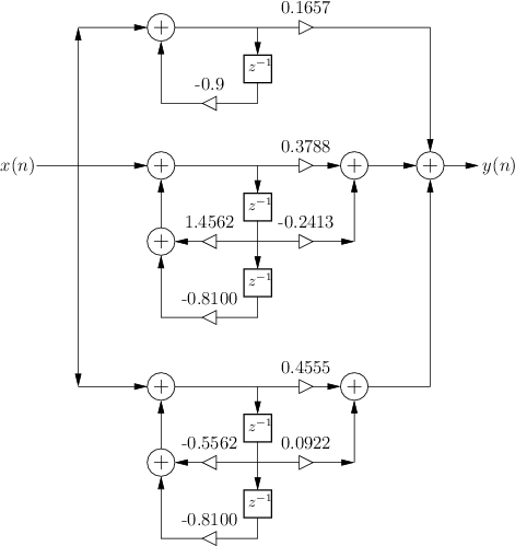
Figure 3.25 shows the signal flow graph for the implementation of our
example filter using parallel second-order sections (with one
first-order section since the number of poles is odd). This is the
same filter as that shown in Fig.3.1 with ![]() ,
,
![]() ,
, ![]() , and
, and ![]() . The second-order sections are
special cases of the ``biquad'' filter section, which is often
implemented in software (and chip) libraries. Any digital filter can
be implemented as a sum of parallel biquads by finding its transfer
function and computing the partial fraction expansion.
. The second-order sections are
special cases of the ``biquad'' filter section, which is often
implemented in software (and chip) libraries. Any digital filter can
be implemented as a sum of parallel biquads by finding its transfer
function and computing the partial fraction expansion.
 |
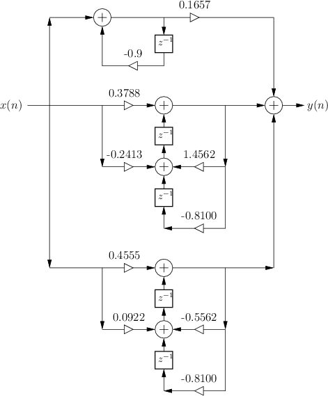 |
The two second-order biquad sections in Fig.3.25 are in so-called ``Direct-Form II'' (DF-II) form. In Chapter 9, a total of four direct-form filter implementations will be discussed, along with some other commonly used implementation structures. In particular, it is explained there why Transposed Direct-Form II (TDF-II) is usually a better choice of implementation structure for IIR filters when numerical dynamic range is limited (as it is in fixed-point ``DSP chips''). Figure 3.26 shows how our example looks using TDF-II biquads in place of the DF-II biquads of Fig.3.25.
Next Section:
Series, Real, Second-Order Sections
Previous Section:
Parallel, Real, Second-Order Sections


